NanoDreamer: A 750k-Parameter World Model That Learns to Act Through Imagination

Benjamin Bai likes video games and had started reading about world models and embodied intelligence, so Dreamer was an obvious attractor. He also had a problem: no GPU. His response was not to wait for hardware. He built a tiny Dreamer from the bottom up: an autograd engine, tensor library, neural-network layers, optimizers, and transformer, all small enough to train on a MacBook.

The result is NanoDreamer, a roughly 750,000-parameter world model and actor-critic that learns to play all five MinAtar games. Each game gets separate weights, but every run uses the same architecture and training recipe. There are no expert demonstrations and no hand-coded strategies. The policy learns from its own gameplay, and the actor trains entirely inside the model's imagined rollouts. At 500,000 policy steps per game, training takes about three hours on an M5 Pro.

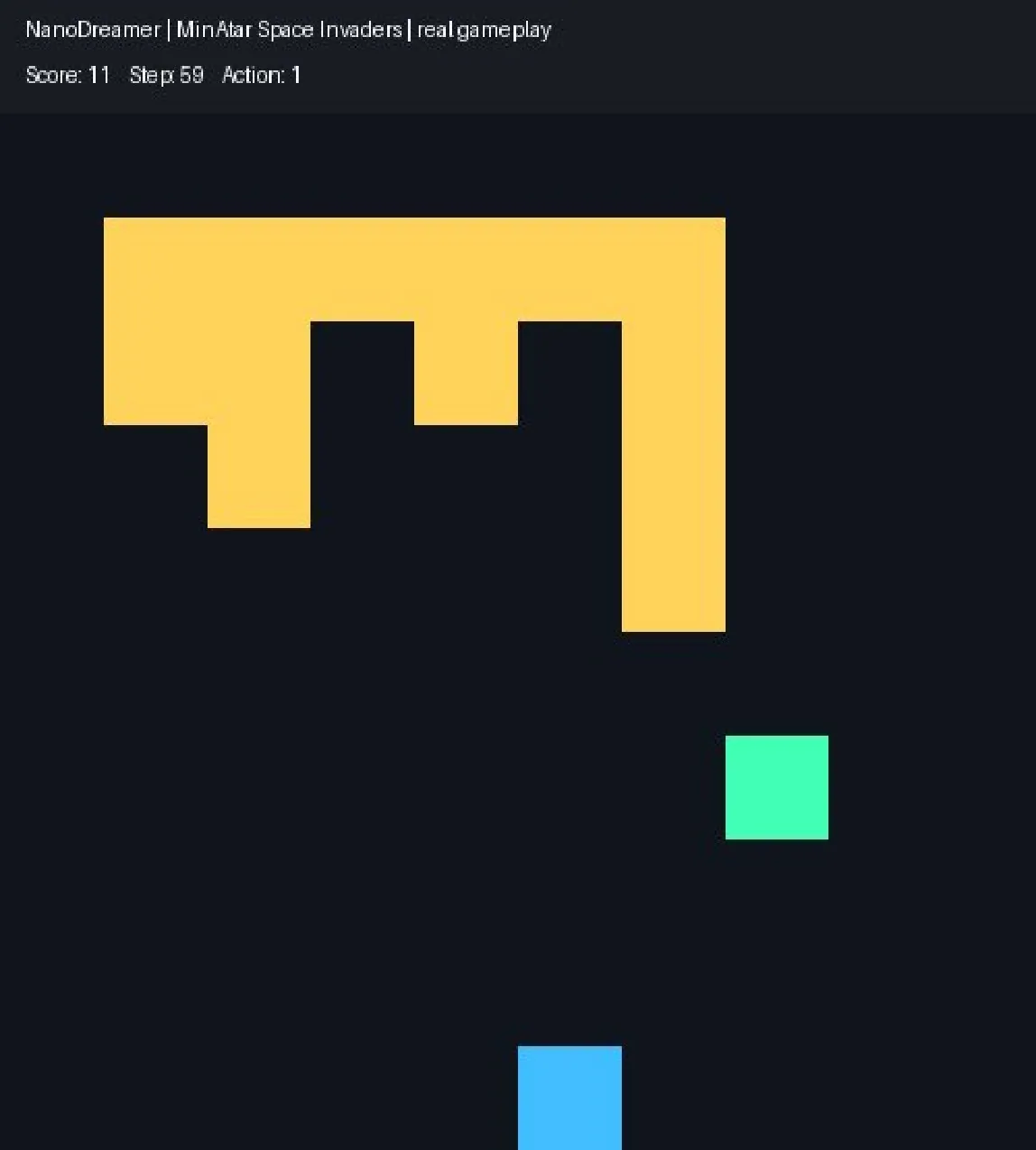
This article is an adapted full translation of Benjamin Bai's write-up. It keeps the failed first attempt visible rather than starting from the final architecture, because the debugging path is where the project's useful lessons live.

The first attempt

Bai began with DreamerV3 and DreamerV4, then reduced the idea to three parts. A world model learns how the game works. An actor chooses actions inside the model's predictions. A critic estimates value beyond the short imagined horizon.

flowchart LR
    F["Game frame"] --> E["MLP encoder
64-D latent"]
    E --> H["Latent history"]
    H --> T["Causal transformer
8 steps"]
    A["Actor action"] --> T
    T --> P1["Next latent"]
    T --> P2["Scalar reward"]
    T --> P3["Continuation probability"]
    H --> AC["Actor / critic MLPs"]
    P1 --> R["5-step imagined rollout"]
    P2 --> R
    P3 --> R
    R --> AC

The first encoder was an MLP autoencoder that compressed a frame into 64 dimensions. Once it could reconstruct the screen, its weights were frozen. Most MinAtar cells are empty, so a reconstruction loss dominated by empty cells can be minimized by predicting a mostly blank screen. The author therefore used weighted binary cross-entropy, making a missed occupied cell more expensive:

$$ \mathcal L_{\mathrm{reconstruction}} =-\operatorname{mean}_i\left[ w_i x_i\log \hat x_i+ (1-x_i)\log(1-\hat x_i) \right]. $$

Here $x_i$ is the real occupancy of one cell in one channel, $\hat x_i$ is its predicted probability, and $w_i$ increases the weight of rare occupied cells. If $x_i=1$, the loss term is $-w_i\log \hat x_i$. Predicting 0.9 costs about $0.105w_i$, while predicting 0.1 costs about $2.303w_i$.

The predictor read eight steps of latent and action history through two causal transformer blocks of width 64 and four attention heads. Three heads predicted the next latent, reward, and continuation:

$$ \hat z_{t+1}=z_t+\Delta z_t, \quad \mathcal L_{\mathrm{next\ latent}} =\mathrm{MSE}(\hat z_{t+1},E(x_{t+1})), $$

$$ \mathcal L_{\mathrm{reward}}=\mathrm{MSE}(\hat r_t,r_t), \qquad \mathcal L_{\mathrm{continuation}}=\mathrm{BCE}(\hat c_t,c_t). $$

The predicted latent was also decoded and compared with the real next frame, with changed cells weighted more heavily so a small moving projectile could not be ignored. The prototype world-model loss was

$$ \mathcal L_{\mathrm{world}} =\mathcal L_{\mathrm{next\ latent}} +2\mathcal L_{\mathrm{reward}} +0.2\mathcal L_{\mathrm{continuation}} +0.5\mathcal L_{\mathrm{predicted\ frame}}. $$

The coefficients were manual balancing weights, not values derived from Dreamer or established as optimal. Because the terms have different numerical scales, the factor of 2 did not mean reward was literally twice as important.

The actor started from real replay history, chose an action, consumed the model's predicted next latent, chose again, and repeated the process for five imagined actions. A simplified return target is

$$ G_0=\hat r_0+\gamma\hat r_1+\gamma^2\hat r_2+\gamma^3\hat r_3 +\gamma^4\hat r_4+\gamma^5V(s_5). $$

The actual implementation used $\lambda$-returns:

$$ G_t^\lambda=\hat r_t+\gamma\hat c_t \left[(1-\lambda)V(s_{t+1})+\lambda G_{t+1}^\lambda\right], \qquad G_5^\lambda=V(s_5). $$

The author used $\gamma=0.99$ and $\lambda=0.95$. The continuation estimate removes future reward when the imagined episode is expected to end. Each decision received its own return target, and the advantage subtracted the critic's expectation:

$$ A_t=\operatorname{sg}(G_t^\lambda-V(s_t)), $$

$$ \mathcal L_{\mathrm{actor}} =-\mathbb E_t[\log \pi(a_t\mid s_t)A_t], \qquad \mathcal L_{\mathrm{critic}} =\mathbb E_t[(V(s_t)-\operatorname{sg}(G_t^\lambda))^2]. $$

A positive advantage made the sampled action more likely; a negative advantage made it less likely. Stop-gradient markers kept the target fixed during an update, and an entropy bonus encouraged exploration. But fitting imagined returns does not guarantee that they match reality.

It did not work

The first run used about 20,000 steps and did not even shoot. Across 30 games it averaged 0.03 points, while a random policy scored 4.3. The agent moved left and right until it lost with zero points.

The first diagnostic was reward prediction. Bai replayed identical actions in the real game and in the learned model, then compared actual and predicted transitions. In one example, the model expected about 1.19 points on step four; the real shot scored one point on step five, exactly where the model predicted almost nothing. It even predicted small negative rewards when no reward occurred.

Across more trajectories, reward timing degraded rapidly as the model rolled forward. On one-step predictions, about 72% of reward events were placed on the correct step. By eight steps, only about 1% were.

Prediction step	Correctly timed reward events	Rate
1	83 / 116	72%
3	23 / 128	18%
5	23 / 124	19%
8	1 / 121	1%

Unreliable imagined rewards could also distort the critic. In one diagnostic, its average value estimate was 10.46, while the average real discounted return was 3.16. The actor was therefore receiving both misplaced rewards and an overly optimistic baseline.

Changing how the model learned

The model could start from a real history but struggled once it had to continue from its own predictions. Bai made two changes. First, he added the actor's real gameplay to replay instead of training only on random experience. The loop became: play a real game, save trajectories, update the encoder and world model, then let the actor and critic practice in imagination. As the policy changed, its new mistakes entered the training data.

Second, he tested multi-step prediction. Instead of only predicting one step from a real history, each predicted latent was fed back into the model. Recorded actions conditioned the rollout, and predictions were compared with the real future latents. In one experiment, the model was fine-tuned for 600 updates on five-step rollouts:

$$ \mathcal L_{\mathrm{rollout}}^{\mathrm{latent}} =\mathrm{error\ at\ step\ 1} +\mathrm{error\ at\ step\ 2} +\cdots +\mathrm{error\ at\ step\ 5}. $$

In a separate five-step check, 600 rollout updates reduced latent prediction error by about 18% and reward prediction error by about 9%. Better predictions did not automatically produce a better agent. When online replay and rollout training were combined, Space Invaders reached about 4 points in 50k steps and then plateaued, still close to the random policy.

Rebuilding representation and rollouts

Bai returned to older DreamerV2 ideas and used the diagnostics to redesign how the model represented screens and practiced futures. A projectile can appear in any column, so an MLP has to learn each position separately. A CNN can reuse the same local filters across the board. The flat-image-plus-MLP encoder became shared 3-by-3 convolutional filters.

The predictor also needed to practice on its own outputs. The rebuild kept three-step generated rollouts and sampled rare reward events more often, with importance weights correcting the biased sampling mixture.

To test whether this helped, Bai replayed identical actions through the early and rebuilt Space Invaders models. Both started from eight real frames and predicted eight steps. The evaluation used trajectories from 30 random-play games and 1,314 rollout windows.

Prediction step	First draft	Rebuilt model
1	53 / 93 = 57%	81 / 93 = 87%
3	21 / 97 = 22%	53 / 97 = 55%
5	6 / 95 = 6%	40 / 95 = 42%
8	0 / 93 = 0%	26 / 93 = 28%

The rebuilt model improved timing and reward totals. Five-step cumulative reward error fell from 0.313 to 0.125, about 60% lower. It was not uniformly better: false alarms at step five increased from 6 to 27. It found more real rewards but also predicted more rewards that never happened.

There was also a perceptual surprise. For one particular shot, the first draft's decoded frames happened to look closer to the real game than the rebuilt model's frames, even though the rebuilt model predicted reward timing much better over the larger test. A cleaner-looking imagined screen was not the same as a more useful reward prediction.

The final recipe

Better predictions only matter if the actor can learn from them, so the final version also changed behavior learning. The actor and critic no longer saw only the current latent plus a one-frame change. They received the transformer's summary of up to 16 frames and preceding actions. A separate action MLP combined the history summary with the chosen action before the prediction heads ran, letting the actor choose from history before the model predicts that action's consequences. The critic also added real replay returns alongside imagined returns to ground its earlier optimism.

flowchart LR
    X["MinAtar frames"] --> C["CNN encoder
16-32-64 channels"]
    C --> Z["64-D latent"]
    Z --> H["Latent and action history
up to 16 steps"]
    H --> T["Causal transformer
width 128, 2 blocks, 4 heads"]
    T --> S["History summary h_t"]
    S --> A["Actor"]
    S --> V["Distributional critic"]
    S --> M["Action MLP"]
    A --> AT["Selected action"]
    AT --> M
    M --> L1["Next latent head"]
    M --> L2["255-bin reward head"]
    M --> L3["Continuation head"]
    L1 --> D["Decoder and predicted frame"]
    L1 --> I["Imagined rollout
5 actions"]
    L2 --> I
    L3 --> I
    I --> A
    I --> V

The CNN encoder compresses each frame to 64 numbers. Its decoder reconstructs the observation channels with weighted binary cross-entropy. Unlike the first draft, prediction losses also update the encoder. A slowly moving target encoder supplies latent targets so the predictor does not chase every encoder update:

$$ \bar\theta_E \leftarrow 0.99\,\bar\theta_E+0.01\,\theta_E. $$

The bar denotes target-encoder weights. Each update keeps 99% of the old target and takes 1% of the current encoder. Gradients do not update the target network.

The transformer reads up to 16 frames and preceding actions. It has two causal blocks, width 128, and four attention heads. A small MLP combines its summary $h_t$ with the current action before three heads predict the next latent, a reward distribution, and continuation probability. For generated step $k$,

$$ \begin{aligned} \ell_k={}&\mathcal L_{\mathrm{next\ latent}} +\mathcal L_{\mathrm{predicted\ frame}}\\ &+2\mathcal L_{\mathrm{reward}} +0.2\mathcal L_{\mathrm{continuation}}. \end{aligned} $$

Next-latent prediction is mean squared error against the target encoder. Predicted-frame loss is weighted binary cross-entropy. The reward head uses cross-entropy against a two-hot target. A symlog transform maps rewards into the range $[-5,5]$, and probability mass is split between neighboring bins:

$$ \operatorname{symlog}(r) =\operatorname{sign}(r)\log(1+|r|), \qquad b=\frac{\operatorname{symlog}(r)+5}{10}\times254. $$

Continuation uses binary cross-entropy. Three generated steps feed their predictions back into the model, one quarter of sampling draws start at reward events, and importance weights correct the induced mixture. The world-model objective is

$$ \mathcal L_{\mathrm{world}} =\mathcal L_{\mathrm{reconstruction}} +\mathcal L_{\mathrm{one\text{-}step}} +\frac13\sum_{k=1}^{3}\ell_k. $$

Reconstruction checks real frames. The one-step term checks latent and decoded-frame predictions from real histories. The averaged three-step term checks futures generated through the model's own outputs. Target latents are detached.

The actor and critic read the transformer's history summary. Starting from replay, the actor chooses five imagined actions. The model predicts each reward and continuation probability, and a target critic estimates what comes after the rollout:

$$ \begin{aligned} G_t^\lambda&=\hat r_t+\gamma\hat c_t \left[(1-\lambda)\bar V(h_{t+1})+\lambda G_{t+1}^\lambda\right],\\ G_5^\lambda&=\bar V(h_5). \end{aligned} $$

As before, $\gamma=0.99$ discounts the future and $\lambda=0.95$ mixes the next critic estimate with the longer return. The actor objective scales the advantage by a running return range $S$ and adds a small entropy bonus:

$$ \begin{aligned} A_t&=\operatorname{sg}\left( \frac{G_t^\lambda-V(h_t)}{\max(1,S)} \right),\\ \mathcal L_{\mathrm{actor}} &=-\mathbb E_t\left[ w_t\left(A_t\log\pi(a_t\mid h_t)+0.001\mathcal H\right) \right]. \end{aligned} $$

Here $w_t$ discounts later states using predicted continuation, and $\mathcal H$ is policy entropy. Actor gradients pass through action probabilities, not through the world model. The critic uses three-step real replay returns plus a smaller imagined-return loss:

$$ \mathcal L_{\mathrm{critic}} =\mathcal L_{\mathrm{real\ replay}} +0.3\,\mathcal L_{\mathrm{imagined}}. $$

Both terms fit distributional value bins to detached two-hot targets. Real examples receive replay importance weights; imagined examples receive continuation weights. The target critic moves 2% toward the current critic per update.

Training begins with 4,000 random environment actions. After that, the actor keeps collecting real gameplay. One world-model, actor, and critic update runs every eight policy steps. Random-action exploration starts at 40% and falls to a 5% floor by 26,250 policy steps, preserving some chance to test actions outside the current preference.

Results across five games

The first promising learning curves came from Space Invaders and Breakout at 200k policy steps. Space Invaders reached 12.87 versus a 4.51 random baseline, almost 3 times random. Breakout reached 3.04 versus 0.44, almost 7 times random.

Bai then trained all five MinAtar games for 500,000 policy steps each with separate weights but identical architecture and hyperparameters. Final scores below are averaged over 100 fresh games per agent, with a 1,000-action limit.

Game	Random baseline	NanoDreamer
Space Invaders	4.14	22.61
Breakout	0.37	5.03
Asterix	0.40	1.50
Seaquest	0.28	3.93
Freeway	0.15	11.23

The same small architecture beat random on every game. Scores are not cross-game comparable because each environment offers different reward opportunities. The 32-point Space Invaders clip shown by the author is a selected episode, not the average.

Ablations and honest limits

The author did not present the final recipe as a set of obviously necessary parts. After the long runs, he removed or changed individual training signals while keeping the actor's imagination-only training fixed. All comparisons used 150,000 real policy steps, 100 evaluation games, and a 200-action limit.

Question	Comparison	Observed result
Should prediction errors train the encoder?	Joint encoder versus reconstruction-only encoder	In seed 0, reconstruction-only scored higher on Space Invaders, 11.26 versus 9.32, and nearly matched Breakout, 2.98 versus 2.92.
Does the critic need real returns?	Full mixed critic versus imagination-only critic	Imagination-only improved both Space Invaders seeds, 15.82/15.14 versus 9.32/11.16, but was seed-dependent on Breakout, 4.82/1.40 versus 2.92/1.48.
Do simpler choices combine well?	Full recipe versus imagined critic versus plus reconstruction encoder, seed 1	Space Invaders: 11.16, 15.14, 12.59. Breakout: 1.48, 1.40, 5.08.

The combination of a reconstruction-only encoder and imagination-only critic reached 5.08 on Breakout while the first two recipes stayed around 1.4-1.5. On Space Invaders it beat the full recipe but remained behind the imagination-only critic with a jointly trained encoder. The effects were not additive, and the combined variant had only one seed.

Architecture searches were also inconclusive. Increasing transformer width from 64 to 128 and blocks from 2 to 3 grew the world model from roughly 109,000 to 613,000 parameters. Some reward metrics improved, but gameplay did not improve consistently. A small RSSM trial, spatial-token experiments, and a denoising experiment attempted to preserve local detail or model more complicated futures, but different checkpoints and short runs prevented a clean architectural conclusion. In one RSSM replay bug, windows requiring eight steps discarded short episodes; in one random dataset, 231 of 300 episodes were too short. The rebuilt replay keeps short terminal windows and masks padding.

Setting	Value
Latent size	64
CNN channels	16 → 32 → 64, 3 × 3 filters
Transformer	Width 128, 2 blocks, 4 heads
History context	16 steps
Reward / value distributions	255 bins, symlog range -5 to 5
World-model / real-return horizon	3 steps
Actor imagination horizon	5 steps
World-model batch	32 replay contexts
Imagination batch	64 starting contexts
Initial random experience	4,000 environment actions
Update frequency	1 update per 8 policy steps
Replay capacity	200,000 transitions
Reward-event sampling	25% event starts + 75% uniform starts, importance corrected
Optimizer	Adam
Learning rates	World 0.0002, actor 0.00004, critic 0.0001
Gradient clipping	Norm 5 for each optimizer
Discount / return mixing	γ = 0.99, λ = 0.95
Actor entropy coefficient	0.001
Policy probability mixing	99% learned probabilities + 1% uniform
Random-action exploration	40% initially, falling to 5% by 26,250 policy steps
Target encoder / critic update	1% / 2% per update
Generated-step loss weights	Latent 1, frame 1, reward 2, continuation 0.2
Critic loss weights	Real replay 1, imagined 0.3

MinAtar rewards were used without custom shaping. There are no extra points for firing, moving, or surviving. Sampling reward events more often and binning rewards change how training data and predictions are formed; neither adds reward to the environment. Rollout and evaluation limits can also end a recorded episode before the environment's own timer, especially in Freeway, whose timer exceeds the 1,000-action final evaluation limit.

Result	Evaluation setup
Longer-run learning curves	100 games per checkpoint, 200-action limit, different evaluation seeds at each checkpoint
Final five-game table	500k training steps, 100 fresh games per game, 1,000-action limit
Training-choice charts	Matched 150k training steps, 100 games, evaluation seed 920000, 200-action limit
Training-choice endpoint checks	300 games, evaluation seed 940000, 200-action limit; one run ended at 184,712 training steps

These results come from one training seed per game in the final table and one or two seeds in auxiliary comparisons. More evaluation games reduce uncertainty about a saved policy, but they do not establish reliability across training seeds.

What transferred beyond the score table

The project changed how Bai reads papers. Architecture diagrams are no longer the primary object of attention; assumptions, training data, diagnostics, and the actual experiment behind a claim matter more. He also separates two achievements that often blur together: making an agent work and understanding why it works. NanoDreamer reached the first. The second remained open.

The next questions are concrete: what information does a 64-dimensional latent discard, when does an imagined rollout become unreliable, and can an agent recognize that unreliability before trusting its own imagination? Bai also leaves open the more playful path: build more working algorithms through favorite video games, including Smash Ultimate or Deadlock.

Source: Benjamin Bai, NanoDreamer: Learning to Act Through Imagination, October 2026. Code: benyebai/NanoDreamer. This is a full bilingual adaptation published with source attribution.