PAPER DEEP DIVE
SparseDrive: End-to-End Autonomous Driving via Sparse Scene Representation
SparseDrive unifies detection, tracking, online mapping, prediction, and planning with sparse scene representation, using a symmetric perception module, a parallel motion planner, and collision-aware rescoring for safe planning.
Paper Metadata
Title: SparseDrive: End-to-End Autonomous Driving via Sparse Scene Representation
Authors: Wenchao Sun, Xuewu Lin, Yining Shi, Chuang Zhang, Haoran Wu, Sifa Zheng
Venue: ICRA 2025; arXiv:2405.19620v2
Paper: https://arxiv.org/abs/2405.19620
Code: github.com/swc-17/SparseDrive (official implementation, models and weights released)
One-Sentence Summary
SparseDrive replaces expensive bird's-eye-view features with a fully sparse scene representation in which detection, tracking, online mapping, motion prediction, and planning share instance-level structure, and a collision-aware rescoring module selects a safe multi-modal plan.
Background and Motivation
Conventional autonomous driving stacks perception, prediction, and planning as separate modules. Each module consumes the output of the previous one, so errors such as a missed object or a coarse velocity estimate propagate forward. This architecture is easy to debug and monitor, but it cannot recover information that was discarded at an earlier stage. The result is a system whose planning quality is bounded by the quality of its intermediate representations.
End-to-end learning addresses this problem by putting all tasks into one differentiable model. UniAD demonstrated that a query-based model can jointly optimize perception, prediction, and planning. VAD showed that vectorized scene representation can reduce the dependence on dense BEV feature maps. Nevertheless, SparseDrive's authors identify two persistent weaknesses: existing methods still rely on computationally expensive BEV features, and their motion prediction and planning branches are often designed in a straightforward sequential manner.
The paper highlights three parallels between prediction and planning that prior methods neglect. First, both tasks must anticipate future trajectories and therefore need high-order bidirectional interaction among road agents; a sequential planner cannot model how the ego vehicle's future behavior affects surrounding vehicles. Second, both tasks need semantic scene understanding and geometric motion cues, but previous models extract those properties for surrounding agents while leaving the ego vehicle without a comparable semantic and geometric instance. Third, both prediction and planning are inherently multi-modal, yet many planners output only one deterministic trajectory.
SparseDrive therefore adopts a Sparse-Centric paradigm. Instead of building a dense BEV tensor, it maintains a set of sparse 3D anchors. Each anchor is paired with an instance feature, and the anchor is iteratively refined by sampling features from multi-view images and attending to other agents. This representation is not a shortcut around perception; it is a common data structure that can support detection, tracking, online mapping, motion prediction, and planning.
The design objective is also broader than accuracy. The paper treats planning safety as a first-class evaluation target. A planner that produces a smooth trajectory but occasionally collides is not useful, so SparseDrive combines multi-modal planning with a hierarchical selection strategy that explicitly rescues unsafe modes before the final trajectory is emitted.
It is useful to quantify what the BEV-centric design costs. A dense BEV feature usually has spatial resolution on the order of hundreds by hundreds, and every camera frame must be projected and splatted into that grid. Temporal fusion then requires aligning and aggregating multiple dense feature maps. The cost grows with resolution and history length even when only a handful of objects matter. Sparse anchors avoid most of this work: each anchor projects a limited set of sampling points into the relevant image views, and temporal alignment operates on anchors rather than on the full grid.
The related-work discussion also shows how the field has moved. PETR replaces geometric projection with positional encoding and global attention. Sparse4D makes anchors explicit and refines them iteratively. MapTR represents map elements as permutation-equivalent point sets. SparseDrive absorbs these ideas into one system. Detection, mapping, and planning no longer need separate scene encoders, and the sparse anchor is the common currency between perception and prediction.
Preliminaries
The Sparse4D line of detectors avoids dense BEV features by using explicit 3D anchors. Each anchor carries position, size, orientation, and velocity, projects into image views, samples local features, and is refined across decoder layers. SparseDrive generalizes this idea: anchors become a universal representation for dynamic agents and static map elements, not merely detection proposals.
End-to-end tracking can be implemented with an instance queue. Detection outputs are matched against the previous frame's instance identities, and matched features and anchors are propagated through time. This removes the separate data-association stage used by tracking-by-detection systems. The same queue also provides temporal context for the motion planner.
Motion prediction and planning share a similar mathematical interface: both map a scene state to a set of future trajectories and confidence scores. They differ in the object being predicted, the prediction horizon, and the downstream safety constraints. SparseDrive exploits this similarity by giving both tasks a shared interaction encoder and separate output heads only at the final refinement layer.
On nuScenes, the evaluation itself is open-loop. Planning is scored by comparing the predicted ego trajectory with recorded future states, and collision rate is measured by checking whether the predicted trajectory overlaps any obstacle. This setup is standard in the end-to-end driving literature, but it places a large burden on the trajectory-selection mechanism because there is no closed-loop controller to recover from a bad local decision. The collision metric therefore deserves careful implementation, which is one reason the paper redefines how boxes are checked.
Method
Input and Overall Architecture
The multi-view image input is written as
$$I=\left\{I_{s}\in\mathbb{R}^{N\times C\times H_{s}\times W_{s}}|1\leq s\leq S\right\},$$where $N$ is the batch size, $C$ is the channel dimension, $S$ is the number of cameras, and $H_s$, $W_s$ define the spatial resolution of camera $s$. A ResNet backbone and an FPN neck encode the images into multi-scale feature maps. The rest of the model consumes those feature maps through sparse anchors instead of dense grid features.
The full pipeline is: encode images, learn a sparse scene representation through symmetric sparse perception, then run motion prediction and planning in parallel. A hierarchical selection stage produces the final safe ego trajectory.
flowchart TB
    A["Multi-view images I"] --> B["Multi-scale features"]
    B --> C["Symmetric sparse perception"]
    C --> D["Detection Fd Bd"]
    C --> E["Online mapping Fm Lm"]
    C --> F["Instance queue tracking"]
    D --> G["Ego init Fe Be"]
    F --> H["Parallel motion planner"]
    G --> H
    H --> I["Motion modes tau_m s_m"]
    H --> J["Planning modes tau_p s_p"]
    I --> K["Hierarchical selection"]
    J --> K
    K --> L["Collision-aware rescore"]
    L --> M["Final safe trajectory tau_p*"]
Symmetric Sparse Perception: Detection
The detection branch uses $N_d$ learned instances. A detection feature $F_{d}\in\mathbb{R}^{N_{d}\times C}$ and an anchor $B_{d}\in\mathbb{R}^{N_{d}\times 11}$ jointly represent a dynamic agent. The 11 anchor dimensions are
$$\left\{x,y,z,\ln w,\ln h,\ln l,\sin{yaw},\cos{yaw},v_x,v_y,v_z\right\}.$$Anchors project onto multi-view feature maps to sample local appearance. A stack of decoder layers then refines each anchor. The last decoder layer produces the final box and class score, while intermediate boxes from earlier layers are also supervised. This iterative refinement is inherited from sparse 3D detection and gives the perception module a stable starting point for planning.
In the released code, the detection head is implemented as `Sparse4DHead`. Its operation order includes `temp_gnn`, `gnn`, `deformable`, `ffn`, and `refine`. The `refine` operation is `SparseBox3DRefinementModule`, which adds an anchor embedding to the instance feature, predicts residuals, and adds those residuals back to the anchor state.
The detection instance bank is configured with 900 anchors. The anchors are generated offline by k-means over the training set so that their spatial distribution matches the data. A separate set of 600 temporal instances is maintained for history, and confidence decay is applied to historical features. The anchor encoder uses separate MLPs for position, size, yaw, and velocity, then concatenates the embeddings when decoupled attention is enabled. This makes it possible to route position and appearance through different attention channels.
The decoder has six layers. The first layer performs single-frame refinement, and the remaining five layers include temporal attention. Each transformer block uses `temp_gnn`, `gnn`, normalization, deformable feature aggregation, feed-forward layers, and a refinement head. The use of FlashAttention and a custom deformable aggregation operator keeps the model efficient enough for multi-task training on a single research GPU setup.
Symmetric Sparse Perception: Online Mapping
The mapping branch represents a map element as an ordered point sequence. Map features are $F_{m}\in\mathbb{R}^{N_{m}\times C}$, and map anchors are $L_{m}\in\mathbb{R}^{N_{m}\times N_{p}\times 2}$, where $N_p$ is the number of sampled points. Each map element is written as
$$\left\{x_{0},y_{0},x_{1},y_{1},\ldots,x_{N_{p}-1},y_{N_{p}-1}\right\}.$$Lane dividers, road boundaries, and pedestrian crossings are output as vectorized point sets. The map decoder uses the same symmetric structure as the detection decoder, so the scene has one model family rather than a separate segmentation and vectorization stack.
In the code, `SparsePoint3DEncoder` embeds a fixed number of sample points, and `SparsePoint3DRefinementModule` predicts offsets that are added to the anchor point set. The map head uses Hungarian matching against ground-truth point sequences. Map instances also participate in cross-attention inside the motion planner, so the planner can distinguish drivable space, lane structure, and static boundaries without an explicit occupancy map.
Symmetric Sparse Perception: Tracking and the Instance Queue
Tracking is handled through identity-aware temporal propagation. Current-frame detection instances are matched to the previous frame by instance ID. Matched features and anchors are reweighted and carried into the current representation, and the queue provides history for temporal attention.
The code config uses 900 detection anchors in the instance bank. The motion-planning head selects the top 50 dynamic instances and top 10 map instances by confidence. Tracking requires no separate loss because the identity assignment itself is performed by the matching mechanism, and the low ID-switch numbers reported in the paper indicate that the queue maintains stable tracklets.
The queue length is four, which means the current frame plus three historical frames participate in temporal modeling. Each frame stores the current instance features, anchors, ego features, and ego anchors. When the vehicle moves, historical anchors are projected from the previous coordinate frame to the current frame using ego motion before attention is applied. This projection is visible in `InstanceQueue.get`, where `anchor_handler.anchor_projection` transforms every cached anchor with the relative pose.
Ego Instance Initialization
The planner must give the ego vehicle the same semantic and geometric treatment as surrounding agents. SparseDrive constructs the ego instance from the smallest front-camera feature map:
$$F_e={\rm AveragePool}(I_{front,S}),$$where $I_{front,S}$ is the finest semantic feature map from the front camera at the coarsest scale. The pooled feature $F_e\in\mathbb{R}^{1\times C}$ summarizes scene context while also serving as dense-feature compensation for obstacles that sparse perception might miss. The ego anchor $B_e\in\mathbb{R}^{1\times 11}$ is initialized from a fixed vehicle box and ego state.
In `instance_queue.py`, `prepare_planning` applies an `ego_feature_encoder` containing convolutions, batch normalization, ReLU, and average pooling to the front feature map. The code stores `self.ego_anchor` as a fixed box of about 4.08m x 1.73m x 1.56m. This code path directly matches the paper's ego initialization formula.
Parallel Interaction over Agents and Ego
The parallel motion planner treats the ego vehicle as one more participant in scene interaction. Detection instances and the ego instance are concatenated:
$$F_{a}={\rm Concat}(F_{d},F_{e}),\quad B_{a}={\rm Concat}(B_{d},B_{e}).$$The resulting $N_d+1$ instances pass through temporal graph attention, instance graph attention, and cross-attention with map instances. Because the ego appears in the same interaction graph as surrounding agents, motion prediction can condition on plausible future ego behavior, and planning can condition on the reactions of other road users.
The official implementation makes this explicit in `motion_planning_head.py`:
# projects/mmdet3d_plugin/models/motion/motion_planning_head.py
instance_feature_selected = torch.cat(
    [instance_feature_selected, ego_feature], dim=1)
anchor_embed_selected = torch.cat(
    [anchor_embed_selected, ego_anchor_embed], dim=1)
The same shared representation then branches into separate motion and planning queries:
motion_query = motion_mode_query + (
    instance_feature + anchor_embed)[:, :num_anchor].unsqueeze(2)
plan_query = plan_mode_query + (
    instance_feature + anchor_embed)[:, num_anchor:].unsqueeze(2)
This is the core of the parallel design: one interaction encoder, two mode-query families, and one refinement layer that emits both prediction and planning outputs.
The operation order in the motion-planning head is `temp_gnn`, `gnn`, `norm`, `cross_gnn`, `norm`, `ffn`, repeated three times, followed by one `refine` layer. The temporal graph connects current instances to the instance queue. The instance graph computes high-order interactions among all selected dynamic agents and the ego vehicle. The cross graph connects these instances to the selected map elements. This sequence gives the planner both temporal memory and scene structure before any mode-specific output is produced.
Decoupled attention is enabled in the motion head. Query and key position embeddings are concatenated to appearance features, and learned linear projections separate them again after attention. This helps the model combine geometric location and semantic appearance without forcing them to share a single embedding space. The same design appears in the detection head and is a practical detail that supports the paper's emphasis on semantic and geometric information.
Multi-Modal Prediction and Planning
Motion mode queries $MQ_{m}\in\mathbb{R}^{\mathcal{K}_{m}\times C}$ and planning mode queries $MQ_{p}\in\mathbb{R}^{N_{cmd}\times\mathcal{K}_{p}\times C}$ are initialized from k-means anchors. The refinement layer produces
$$\tau_{m}=MLP(F_{d}+MQ_{m}),\quad s_{m}=MLP(F_{d}+MQ_{m}),$$ $$\tau_{p}=MLP(F_{e}+MQ_{p}),\quad s_{p}=MLP(F_{e}+MQ_{p}).$$Here $\tau_m$ denotes the motion trajectories for surrounding agents, $s_m$ their scores, $\tau_p$ the ego planning trajectories, and $s_p$ the planning scores. The number of modes is determined by clustering. Training uses a winner-takes-all strategy: only the trajectory closest to the ground truth receives positive supervision.
The configuration uses `fut_ts=12`, `fut_mode=6`, `ego_fut_ts=6`, and `ego_fut_mode=6`. The `MotionPlanningRefinementModule` has separate branches for motion classification, motion regression, planning classification, planning regression, and ego status. These branches are small MLPs, so the shared interaction layers dominate the computation.
The mode anchors are not arbitrary constants. Motion anchors are selected from a class-conditioned k-means anchor bank, and the anchor for each agent is converted from the agent's local frame to the lidar frame before query generation. Planning anchors are tiled from a fixed ego anchor bank. This initialization gives the mode queries a geometric prior, so the MLP only needs to refine the modes rather than discover them from scratch.
During training, the trajectory with the lowest average displacement error is treated as the positive sample for each agent, while the other modes receive negative supervision. The regression targets are represented as incremental displacements, and the decoder accumulates them over time. This design avoids unstable absolute-coordinate targets and makes the multi-modal outputs easier to compare across agents and horizons.
Hierarchical Planning Selection
Planning outputs are organized by driving command. The first selection level chooses the command, and the second level selects one of the multi-modal trajectories inside that command. This hierarchy reduces the search space and keeps the model aligned with how an ego-command-conditioned planner is evaluated on nuScenes.
The final selection is not a simple argmax over learned scores. A collision-aware rescore module compares candidate ego trajectories with the highest-confidence motion trajectories from surrounding agents. If an ego box overlaps with an obstacle box at any future timestamp, that planning mode receives a large score penalty.
The implementation in `decoder.py` is direct:
# projects/mmdet3d_plugin/models/motion/decoder.py
all_col = col.all(dim=-1)
col[all_col] = False # all modes collide, no need to rescore
score_offset = col.float() * -999
plan_cls = plan_cls + score_offset
The special case for "all modes collide" is important. If every candidate trajectory collides, the module leaves the original scores untouched instead of making all modes equally invalid, which would remove any useful signal for the downstream planner. Rescoring only affects selection and does not rewrite the trajectory, so it remains compatible with end-to-end training.
The rescore module also contains several geometric constants. Ego boxes are expanded by a scale factor of 1.1, the offset for collision checks is 0.5m, static obstacles use a displacement threshold of 0.5m, and motion modes below a confidence threshold of 0.5 are filtered out. The ego yaw is estimated from trajectory points, with a stable default orientation for near-static trajectories. These choices make the geometric check cheap enough to run during inference while still capturing the most important collision cases.
Experiments
Main Results on nuScenes
SparseDrive is evaluated on the nuScenes validation split against modular and end-to-end baselines. SparseDrive-B improves detection, tracking, mapping, prediction, and planning simultaneously. The summary table shows the most important metrics:
| Method | NDS | AMOTA | Map mAP | minADE | L2 Avg | Col Avg | FPS |
|---|---|---|---|---|---|---|---|
| UniAD | 0.498 | 0.359 | - | 0.71 | 0.73 | 0.61% | 1.8 |
| VAD | - | - | 0.476 | - | 0.72 | 0.21% | 4.5 |
| SparseDrive-S | 0.525 | 0.386 | 0.551 | 0.62 | 0.61 | 0.08% | 9.0 |
| SparseDrive-B | 0.588 | 0.501 | 0.562 | 0.60 | 0.58 | 0.06% | 7.3 |
The NDS improvement from 0.498 to 0.588 is large in the context of end-to-end driving. AMOTA rises from 0.359 to 0.501, and ID switches fall from 906 to 632. These gains are especially meaningful because they come from a shared sparse representation rather than from stacking independent task-specific enhancements.
The full detection table also shows consistent regression improvements. UniAD reports 0.380 mAP, 0.684 mATE, 0.277 mASE, 0.383 mAOE, 0.381 mAVE, and 0.192 mAAE. SparseDrive-B reports 0.496 mAP, 0.543 mATE, 0.269 mASE, 0.376 mAOE, 0.229 mAVE, and 0.179 mAAE. The velocity error improves by a relatively large amount, which is sensible because temporal instance propagation gives the model a strong velocity prior.
Tracking numbers tell a similar story. SparseDrive-B reaches 0.501 AMOTA, 1.085 AMOTP, 0.601 Recall, and 632 ID switches, compared with UniAD's 0.359 AMOTA, 1.320 AMOTP, 0.467 Recall, and 906 ID switches. The lower ID-switch count is particularly relevant to the planner because stable tracklets reduce the chance of treating the same vehicle as multiple obstacles or dropping it entirely during a turn.
For mapping, SparseDrive-B reaches 56.2% mAP, including 53.2% on pedestrian crossings, 56.3% on dividers, and 59.1% on road boundaries. VAD reaches 47.6% mAP under the same evaluation. The mapping task still lags dedicated single-task methods, but it is now learned inside the end-to-end model instead of being assumed from an external HD map.
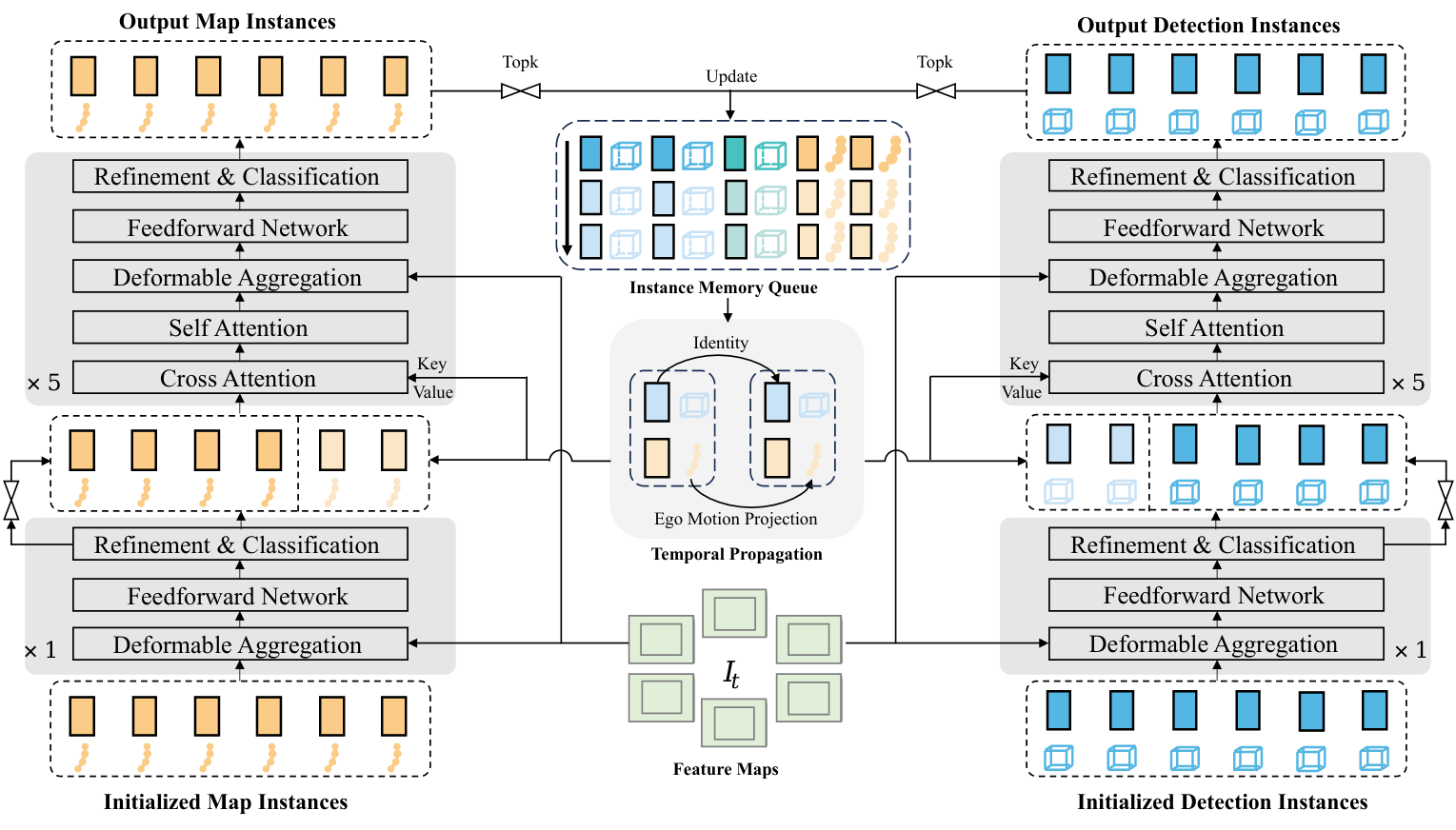
Overview of SparseDrive from Figure 3 of the paper.
Planning Safety and Detailed Metrics
Planning results are reported at 1s, 2s, and 3s horizons. SparseDrive-B achieves 0.58m average L2 error and 0.06% average collision rate, compared with UniAD's 0.73m and 0.61%. The detailed planning comparison is:
| Method | L2 1s | L2 2s | L2 3s | L2 Avg | Col 1s | Col 2s | Col 3s | Col Avg |
|---|---|---|---|---|---|---|---|---|
| UniAD | 0.45 | 0.70 | 1.04 | 0.73 | 0.62% | 0.58% | 0.63% | 0.61% |
| VAD | 0.41 | 0.70 | 1.05 | 0.72 | 0.03% | 0.19% | 0.43% | 0.21% |
| SparseDrive-S | 0.29 | 0.58 | 0.96 | 0.61 | 0.01% | 0.05% | 0.18% | 0.08% |
| SparseDrive-B | 0.29 | 0.55 | 0.91 | 0.58 | 0.01% | 0.02% | 0.13% | 0.06% |
The authors also reimplement the collision metric. Prior implementations rasterized obstacles into a 0.5m occupancy grid and did not account for ego heading change, which can create false collisions near small obstacles. The new metric estimates yaw from trajectory points and checks bounding-box overlap with proper orientation. This makes the safety comparison more reliable.
The prediction results are also strong. SparseDrive-B reaches 0.60m minADE, 0.96m minFDE, 13.2% MissRate, and 0.555 EPA. UniAD reaches 0.71m minADE, 1.02m minFDE, 15.1% MissRate, and 0.456 EPA. The improvement in EPA is notable because it measures whether end-to-end prediction remains useful under a planning-oriented assignment, not just whether trajectories are geometrically close.
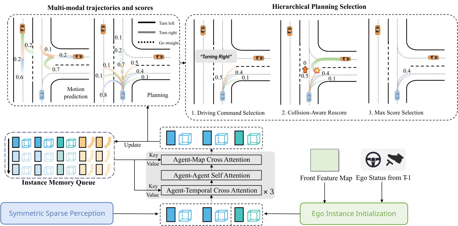
Parallel motion planner architecture from Figure 5 of the paper.
Efficiency
SparseDrive-S runs at 9.0 FPS on a single RTX 4090 and trains in about 20 hours. UniAD runs at 1.8 FPS on a single A100 and requires about 144 hours. SparseDrive-S uses 85.9M parameters and 192G FLOPs, while UniAD uses 125M parameters and 1709G FLOPs. The sparse representation removes dense BEV computation and substantially lowers the cost of experimenting with end-to-end driving.
The released code also reports checkpoint-level numbers under its reimplemented collision metric. The stage-2 SparseDrive-S checkpoint reaches 0.5257 NDS, 56.56% mapping mAP, 37.2% AMOTA, 0.61m minADE, 0.61m planning L2, and 0.097% collision rate. These numbers differ slightly from the paper table because the released evaluation accounts for collision cases that were not considered in the initial code. Reporting both sets of numbers is useful for reproducibility and shows how sensitive open-loop safety metrics can be to implementation details.
Ablation: Components of the Parallel Motion Planner
The paper ablates the parallel design (PAL), ego instance initialization (EII), multiple planning modes (MTM), agent-temporal cross-attention (ATA), and collision-aware rescoring (CAR). Selected results are:
| ID | PAL | EII | MTM | ATA | CAR | minADE | L2 Avg | Col Avg |
|---|---|---|---|---|---|---|---|---|
| 1 | yes | yes | yes | yes | yes | 0.623 | 0.61 | 0.08% |
| 2 | no | yes | yes | yes | yes | 0.641 | 0.61 | 0.10% |
| 3 | yes | no | yes | yes | yes | 0.621 | 0.63 | 0.11% |
| 4 | yes | yes | no | yes | yes | 0.626 | 0.69 | 0.25% |
| 5 | yes | yes | yes | no | yes | 0.634 | 0.77 | 0.16% |
| 6 | yes | yes | yes | yes | no | 0.623 | 0.61 | 0.12% |
Removing parallel interaction raises minADE from 0.623 to 0.641 and collision rate from 0.08% to 0.10%. Removing ego initialization raises L2 from 0.61 to 0.63. Removing multiple planning modes raises collision rate to 0.25%. The largest L2 degradation comes from removing agent-temporal cross-attention: average L2 becomes 0.77m. Each component contributes to a different part of the prediction-planning tradeoff.
Collision-Aware Rescoring versus Post-Optimization
UniAD uses rule-based post-optimization to correct planning outputs. SparseDrive reproduces that strategy and finds it raises L2 from 0.61m to 0.73m while increasing collision rate from 0.25% to 0.61%. The external optimization conflicts with the end-to-end objective and can make the trajectory less safe under the corrected metric.
Collision-aware rescoring instead keeps L2 at 0.61m and reduces collision rate from 0.12% to 0.08%. Because it selects among already generated trajectories rather than rewriting them, the final output remains consistent with the learned planner. This result is one of the clearest demonstrations of why safety should be integrated into the selection stage.
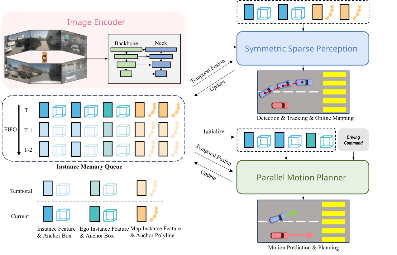
Symmetric sparse perception architecture from Figure 4 of the paper.
Training Objectives
SparseDrive is trained in two stages. Stage one trains symmetric sparse perception from scratch so that the model learns a stable sparse scene representation. Stage two unfreezes all weights and jointly optimizes perception with the parallel motion planner. The total loss is
$$\mathcal{L}=\mathcal{L}_{det}+\mathcal{L}_{map}+\mathcal{L}_{motion}+\mathcal{L}_{plan}+\mathcal{L}_{depth}.$$Detection and mapping losses each combine a classification term and a regression term:
$$L_{det}=\lambda_{det\_cls}L_{det\_cls}+\lambda_{det\_reg}L_{det\_reg},$$ $$L_{map}=\lambda_{map\_cls}L_{map\_cls}+\lambda_{map\_reg}L_{map\_reg}.$$Depth estimation is used as an auxiliary task:
$$L_{depth}=\lambda_{depth}L_{depth}.$$Motion and planning share one combined loss with classification, regression, and ego-status terms:
$$L_{motion\_planning}=\lambda_{motion\_cls}L_{motion\_cls}+\lambda_{motion\_reg}L_{motion\_reg}+\lambda_{plan\_cls}L_{plan\_cls}+\lambda_{plan\_reg}L_{plan\_reg}+\lambda_{plan\_status}L_{plan\_status}.$$The configuration uses $\lambda_{motion\_cls}=0.2$, $\lambda_{motion\_reg}=0.2$, $\lambda_{plan\_cls}=0.5$, $\lambda_{plan\_reg}=1.0$, and $\lambda_{plan\_status}=1.0$. Planning regression receives the largest weight, which expresses the planning-oriented nature of the full pipeline.
Limitations
The authors explicitly state that SparseDrive still trails specialized single-task methods in online mapping. Shared representations help the end-to-end system coordinate multiple tasks, but they may cap the ceiling of any one task. This is an expected tradeoff, yet it matters for deployment because mapping quality has direct consequences for planning.
They also note that the dataset scale is limited and that open-loop evaluation cannot fully represent real driving performance. nuScenes contains valuable scenarios, but it is not large enough to reveal all long-tail interactions. A model that performs well on open-loop L2 and collision metrics may still behave differently under closed-loop control or with distribution shift.
From an implementation perspective, the rescore module is a coarse geometric check. It detects collisions by testing whether corners of one box lie inside another, which is a rough approximation for arbitrary rotated rectangles. The code itself calls this a rough check. Unusual obstacle shapes or very different box sizes could produce missed or spurious collisions.
The rescoring signal also depends on the quality of motion prediction. It uses the most confident predicted modes of surrounding agents. If the true future trajectory has low confidence in the prediction head, the rescore module may not see the relevant obstacle interaction. SparseDriveV2, released after this work, continues to evolve the representation and training pipeline, which suggests that the first version still leaves room for improvement in interaction modeling and evaluation.
Another practical limitation is that all perception and planning modules are trained on camera inputs with an auxiliary depth branch. SparseDrive does not consume lidar or radar as primary inputs. This keeps the system simple and cost-effective, but it also means performance depends on the visual depth quality and camera calibration. Sensor failures, severe weather, and long-tail appearance shifts are not directly addressed by the paper.
Conclusion and Outlook
SparseDrive makes three connected contributions. It replaces dense BEV features with a sparse instance representation that unifies perception tasks; it designs prediction and planning as parallel multi-modal tasks over a shared interaction graph; and it introduces hierarchical selection with collision-aware rescoring for safe trajectory output.
The experiments show simultaneous gains in accuracy, efficiency, and safety. Future directions include stronger single-task perception, larger-scale training, closed-loop evaluation, additional sensors, and more expressive collision reasoning. The open-source implementation and released checkpoints make these extensions practical for the research community.