PAPER DEEP DIVE
Fast-FoundationStereo: Real-Time Zero-Shot Stereo Matching
Fast-FoundationStereo accelerates the three bottlenecks of FoundationStereo separately: distillation compresses the hybrid monocular+stereo backbone into one efficient student, blockwise NAS searches cost-filtering designs under latency budgets with ILP, and structured pruning guided by a recurrent dependency graph slims the ConvGRU refinement module. Trained with 1.4M auto pseudo-labeled in-the-wild stereo pairs, it runs over 10x faster than FoundationStereo while nearly matching zero-shot accuracy, setting a new state of the art among real-time methods on Middlebury, ETH3D, KITTI and Booster.
Paper Info
Title: Fast-FoundationStereo: Real-Time Zero-Shot Stereo Matching
Authors: Bowen Wen, Shaurya Dewan, Stan Birchfield (NVIDIA)
Venue: arXiv:2512.11130v1 (December 11, 2025, cs.CV), CVPR 2026
Paper: https://arxiv.org/abs/2512.11130
Project page: https://nvlabs.github.io/Fast-FoundationStereo/
Code: Open-sourced (NVlabs/Fast-FoundationStereo, PyTorch and TensorRT weights)
In One Sentence
NVIDIA takes the slow-but-strong FoundationStereo, splits it into feature extraction, cost filtering, and disparity refinement, and hits each stage with a different compression tool (knowledge distillation, blockwise neural architecture search, structured pruning), cutting single-frame latency from 496 ms to 49 ms on an RTX 3090 (21 ms under TensorRT) while giving up only a little zero-shot accuracy.
1. Background and Motivation
Stereo matching turns 50 this year, counting from Marr and Poggio's computational theory in 1975. On the standard benchmarks (Middlebury, ETH3D, KITTI) the leading methods are close to saturation, with errors often in the low single-digit percentages. That precision is not academic: robotic grasping, 3D registration for augmented reality, and obstacle ranging for autonomous driving all fail visibly when depth is off by a few pixels.
Over the past few years the field has effectively split into two camps that barely talk to each other. The first is the foundation-model camp. FoundationStereo pairs DepthAnythingV2 as a monocular prior with a side-tuned CNN for the binocular setting; MonSter marries monocular depth to stereo matching; StereoAnywhere targets robustness when either modality fails; ZeroStereo synthesizes training data with diffusion models. These methods generalize zero-shot remarkably well, and they pay for it in compute. They lean on ViT-scale backbones and a Disparity Transformer that runs multi-head self-attention over a 4D cost volume. The authors measure FoundationStereo at 496 ms per frame on a 3090, which rules it out of any latency-constrained system.
The second camp is real-time stereo: IINet, LightStereo, RT-IGEV, BANet. These hit 30 ms per frame with lightweight backbones, 2D convolutions, and local iterative refinement. The catch is that their generalization is almost entirely a product of per-domain fine-tuning. Move to a new scene and you re-collect, re-annotate, and re-train. Dense, high-quality real-world depth ground truth is genuinely hard to obtain at scale, so this camp has never been a drop-in solution for an embodied agent operating outdoors.
The authors argue the gap should not be closed by designing yet another lightweight network trained from scratch. Training from scratch throws away the priors that internet-scale imagery baked into the foundation model, and those priors are precisely where zero-shot generalization comes from. So they invert the problem: treat the powerful FoundationStereo as a teacher and systematically dismantle every compute bottleneck in it while preserving as much of the inherited capability as possible.
The key insight is that the three stages of FoundationStereo bottleneck for completely different reasons. Feature extraction is expensive because of its dual-module hybrid backbone; cost filtering is expensive because of 4D attention; refinement is expensive because of iteration count and channel redundancy. One compression hammer does not fit all three nails, hence the divide-and-conquer strategy: one tailored technique per stage. Figure 1 makes the case visually. The disparity maps are nearly indistinguishable from MonSter and FoundationStereo while running almost 10x faster, and in a few regions (the reflective door in the top row, the paper towel bin in the bottom row) they are actually better than MonSter.
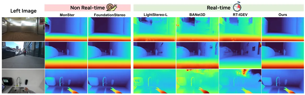
Figure 1: Zero-shot disparity maps on in-the-wild images. The proposed method matches MonSter and FoundationStereo while running nearly 10x faster.
2. Method
2.1 Framework: Divide and Conquer Across Three Stages
A foundation stereo model such as FoundationStereo decomposes into feature extraction, cost filtering, and disparity refinement. The whole method (Fig. 3 in the paper) is organized around those three stages, each accelerated by a different, mutually orthogonal technique that can be swapped independently. This decomposition carries a practical bonus: each stage yields a family of candidate modules at different speed-accuracy points, so deployment becomes an assembly problem. Every starred point in Fig. 2 of the paper is one such assembly, followed by a single end-to-end joint training run.
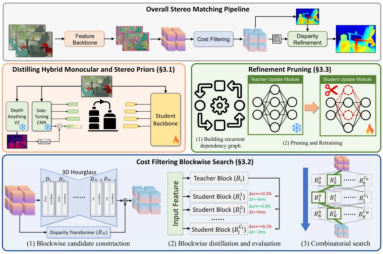
Figure 3: Framework overview. Top: the three key steps of a foundation stereo network. Middle-left: hybrid monocular and stereo priors are distilled into a single student backbone. Middle-right: the refinement network is pruned after constructing a dependency graph that models the recurrent GRU, then retrained to recover accuracy. Bottom: the cost filtering network is split into local blocks, each block candidate is distilled against its teacher counterpart, and combinatorial search picks the best combination under a runtime constraint.
The full pipeline reads as follows:
flowchart TB
    T["Teacher: FoundationStereo
DepthAnythingV2 + side-tuning CNN
3D hourglass APC + Disparity Transformer
ConvGRU refinement"]
    T --> S1
    T --> S2
    T --> S3

    subgraph S1["Stage 1: Feature Extraction -> Knowledge Distillation"]
        A1["Freeze teacher dual-module backbone"]
        A2["Student: EdgeNeXt ImageNet-pretrained CNN"]
        A3["MSE on multi-level pyramid features
linear projection if channel mismatch"]
        A1 --> A3
        A2 --> A3
    end

    subgraph S2["Stage 2: Cost Filtering -> Blockwise NAS"]
        B1["Split into N=8 blocks at channel transitions"]
        B2["5 layer types: 3D conv / 3D deconv /
APC / residual 3D conv / volume excitation"]
        B3["Distill each block independently
200 candidates per block"]
        B4["ILP combinatorial search
min error s.t. runtime budget"]
        B1 --> B2 --> B3 --> B4
    end

    subgraph S3["Stage 3: Refinement -> Structured Pruning"]
        C1["Build recurrent dependency graph
3 stereo-specific constraints"]
        C2["First-order Taylor importance ranking"]
        C3["Prune ratio alpha then retrain
gamma=0.9 decayed L1 + lambda=0.1 feature MSE"]
        C1 --> C2 --> C3
    end

    S1 --> ASM["Assemble candidates + end-to-end training"]
    S2 --> ASM
    S3 --> ASM
    D["Pseudo-labeling pipeline
Stereo4D + normal consistency + sky exclusion
1.4M in-the-wild pairs"] --> ASM
    ASM --> OUT["Fast-FoundationStereo
49 ms on RTX 3090, 21 ms with TensorRT"]
2.2 Stage One: Distilling Hybrid Monocular and Stereo Priors
Given a rectified pair $I_{l}, I_{r} \in \mathbb{R}^{H\times W\times 3}$, the backbone must produce a multi-level feature pyramid for cost volume construction and aggregation:
$$f_{l}^{(i)}, f_{r}^{(i)} \in \mathbb{R}^{C_{i}\times\frac{H}{i}\times\frac{W}{i}}, \quad i \in \{4, 8, 16, 32\}$$
FoundationStereo computes these with two modules working together: DepthAnythingV2 supplies rich monocular priors learned from large-scale internet data, and a side-tuning CNN adapts those monocular features to the binocular stereo setup. The hybrid is powerful, and it is also a major compute bottleneck, because the ViT self-attention underneath it is not cheap.
The authors replace the dual module with a single student module via knowledge distillation, and they are explicit about why. First, distillation is architecture-agnostic, so the student can be drawn from the well-studied family of lightweight ImageNet backbones (EdgeNeXt here). Second, pruning was considered and rejected for two concrete reasons: it would force them to keep the dual module, still shackled to the ViT bottleneck; and any accuracy loss would be hard to recover without retraining on internet-scale imagery, which is exactly the capability source they cannot reproduce from stereo datasets alone.
The distillation recipe is straightforward. Freeze the teacher's DepthAnythingV2 and side-tuning CNN, let them predict the multi-level pyramid $\bar{f}^{(i)}$, and train the student to match it under an MSE loss. Where the channel dimensions disagree, a linear projection layer is inserted. One detail is easy to miss but matters: the feature extractor consumes a single image, yet both stereo images are placed in every training batch so that the feature statistics the student sees during training match those at inference time.
To produce a family of models spanning different speed-accuracy trade-offs, several student variants are trained on ImageNet-pretrained backbones. Figure 4 shows what distillation actually transfers: the student captures high-frequency edges and relative depth similar to the teacher. The more interesting result is the bottom row, where distillation improves robustness to translucency. A translucent glass door is a classic failure case for conventional stereo matching.
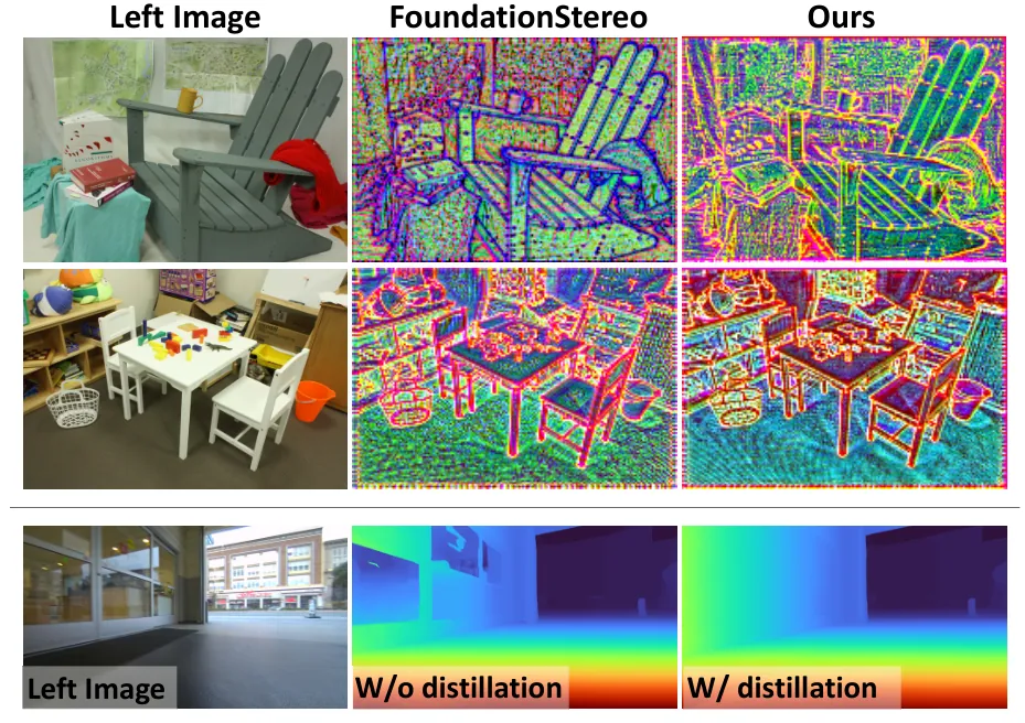
Figure 4: Top: distilling hybrid monocular and stereo priors into a unified single backbone captures similar high-frequency edges and relative depth at far lower compute. Bottom: distillation improves robustness to translucency, a long-standing weakness of conventional stereo matching.
2.3 Stage Two: Blockwise Architecture Search for Cost Filtering
From the unary features, the cost volume is built by combining group-wise correlation and concatenation volumes:
$$\mathbf{V_{C}} \in \mathbb{R}^{C\times\frac{D}{4}\times\frac{H}{4}\times\frac{W}{4}}$$
where $D$ is the maximum disparity (192 by default in this work). FoundationStereo filters this volume with a dual-branch design. One branch is a 3D hourglass built from Axial-Planar Convolution (APC) layers, which enlarges the effective kernel along the disparity axis without a proportional memory increase. The other is a Disparity Transformer that tokenizes $\mathbf{V_{C}}$ and applies multi-head self-attention to strengthen long-range reasoning inside the 4D volume. Both are expensive, the attention branch especially so.
Why neither prune nor directly distill this stage? The authors give two grounded rejections. Direct pruning buys only marginal speedup at severe accuracy cost, because the channel dimension of $\mathbf{V_{C}}$ is already small, mostly under 100, so there is little to remove. Direct distillation would require hand-designing replacement cost-filtering modules, and unlike feature backbones, these structures are not well explored; humans do not have good candidate designs here. So they turn to Neural Architecture Search and let it find designs nobody would propose.
Blockwise candidate construction. The cost filtering module is divided into a chain of operation blocks: $\Phi_{t}(\mathbf{V_{C}}) = B_{N}\circ\cdots\circ B_{2}\circ B_{1}(\mathbf{V_{C}})$, with $N$ blocks total. Inside the 3D hourglass, block boundaries are placed where the channel dimension transitions, which typically coincides with a change in the spatial dimensions of the feature volume. Five layer types are allowed: (1) 3D convolution with variable channel dimensions; (2) 3D deconvolution that doubles the spatial dimensions; (3) APC layers, which convolve the spatial and disparity dimensions separately with different kernel sizes; (4) residually connected 3D convolution layers in the ResNet sense; (5) feature-guided volume excitation. The entire Disparity Transformer is treated as one block made of repeated multi-head self-attention layers, reusing the teacher's disparity attention layers while varying feed-forward dimension, head count, and layer count.
In both cases the number of layers per block and the intermediate channel dimension are free, subject to two constraints: (1) the whole block's runtime $t_{B}^{s}$ must be faster than its teacher counterpart $t_{B}^{t}$; (2) the block's input and output channel dimensions must match the original. Constraint two is what makes blocks pluggable. Fix the interface and each block can be evaluated and replaced in isolation.
Blockwise distillation and evaluation. After construction there are $C = C_{1}\cdot C_{2}\cdots C_{N}$ possible cost filtering candidates. With $N=8$ and $C_{i}=200$, that is $C = 200^{8} \approx 10^{18}$. Standard evolutionary NAS is simply not tractable at that scale, and training from scratch across the whole space wastes the teacher's knowledge. The fix is to train each block $B_{i}$ as a standalone network that mimics its teacher counterpart:
$$\left\| B_{i}(f_{i-1}) - \bar{B}_{i}(f_{i-1}) \right\|^{2}_{2}$$
where $f_{i-1}$ is the feature output from the preceding teacher block. For the final block, which predicts the initial disparity, a smooth $L_1$ loss against ground truth is used instead. The teacher stays frozen throughout. Compared with standard NAS, blockwise distillation reduces training complexity from $O(n^{N})$ to $O(n)$, where $n$ is the number of per-layer candidates. Exponential becomes linear, and this is the cleanest piece of engineering in the paper. Because each block is small, distillation is cheap in both time and memory and parallelizes trivially.
Once distilled, a candidate block $B_{i}^{c}$ is scored by substituting it into position $i$ of the teacher model and running the complete network end-to-end on a held-out validation set, recording the resulting relative error change $\Delta m_{i}^{c}$ and runtime change $\Delta t_{i}^{c}$.
Combinatorial search. The student cost filtering module is the optimal combination of candidate blocks, cast as a constrained optimization:
$$\min_{\mathcal{E}} \sum_{i=1}^{N}(\Delta\mathbf{m}_{i})^{\top}\mathbf{e}_{i}, \quad \text{s.t.} \quad \sum_{i=1}^{N}(\Delta\mathbf{t}_{i})^{\top}\mathbf{e}_{i} \leq \Delta\tau \qquad (1)$$
Here $\Delta\mathbf{m}_{i}$ and $\Delta\mathbf{t}_{i}$ are the vectors of error and runtime changes over all candidates at block $B_{i}$, $\mathbf{e}_{i}\in\mathcal{E}$ is the one-hot selection vector, and $\Delta\tau$ is the runtime budget for the whole cost filtering module relative to the teacher. This is solved by Integer Linear Programming. Sweeping $\tau$ produces an entire family of cost-filtering students at different speed-accuracy points in one pass, which is where the string of stars in Fig. 2 comes from.
2.4 Stage Three: Structured Pruning of the Refinement Module
Given the initial disparity $d_{0}$ from the filtered cost volume and a hidden feature initialized by the context network, a ConvGRU progressively refines the disparity map. Figure 5 shows its dependency graph and data flow: at each iteration the ConvGRU consumes $d_{k-1}$ and $h_{k-1}$ and predicts $d_{k}$ and $h_{k}$, creating recurrent dependencies. The authors quantify this module's redundancy in Sec. 4.4 of the paper. Aggressive pruning degrades accuracy sharply, but retraining recovers it, which is direct evidence that the original refinement module carries a large amount of slack. That motivates structured pruning: simple, effective, and able to benefit from GPU acceleration stacks such as TensorRT.
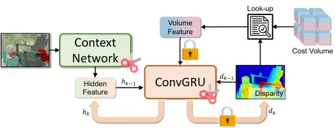
Figure 5: Recurrent dependency graph of the refinement module, marking where pruning is performed and where the channel dimension must remain fixed.
Building the recurrent dependency graph. The first step of structured pruning is identifying inter-layer dependencies, since pruning depth or channels at one layer changes the intermediate feature dimensions fed to its neighbors. Beyond the ordinary adjacent-layer dependencies that can be constructed automatically by tracing the computation flow, the authors add three constraints specific to stereo refinement: (1) inside the ConvGRU, the final layers predicting the disparity map and the convex upsampling mask keep fixed output channel dimensions, because their outputs correspond directly to physical quantities; (2) inside the ConvGRU, the input channels of the layer consuming $h_{k-1}$ and the output channels of the layer producing $h_{k}$ are interdependent and must be pruned jointly, a constraint unique to recurrent structure since $h$ is carried across iterations and must stay dimensionally self-consistent; (3) the motion encoder consuming the indexed volume feature keeps a fixed input channel dimension.
Pruning and retraining. To decide what to remove, importance is estimated by first-order Taylor expansion. Inputs are propagated end-to-end through the full teacher model over multiple refinement iterations, gradients are accumulated for the refinement module, every parameter is ranked globally by importance, and the least important fraction $\alpha\in(0,1)$ is pruned. An isomorphic pruning strategy was also tried and gave slightly worse results, so it was not used.
After pruning, only the refinement module is retrained, with the rest of the teacher frozen, using:
$$\mathcal{L} = \sum_{k=1}^{K}\gamma^{K-k}\left\|d_{k}-\overline{d}\right\|_{1} + \lambda\sum_{i=1}^{L}\left\|x_{i}-\overline{x}_{i}\right\|_{2}^{2} \qquad (2)$$
where $x_{i}$ and $\overline{x}_{i}$ are the student and teacher latent features at each of the $L$ layers, $\overline{d}$ is ground-truth disparity, and $k$ is the iteration index. The factor $\gamma=0.9$ exponentially up-weights later iterations: the closer an iteration is to the final output, the more it matters, and earlier iterations are allowed to be coarser. $\lambda=0.1$ weights the distillation term. One deliberate omission is worth noting: supervision on the initial disparity is excluded, because the refinement module does not affect it, and including it would only inject irrelevant gradient.
2.5 The Fourth Leg: Pseudo-Labeling In-the-Wild Data
Real data offers diversity and realism that synthetic data cannot match, but real stereo images with ground-truth metric depth are notoriously hard to acquire. The authors therefore build an automatic data curation pipeline that pseudo-labels internet-scale stereo imagery (Fig. 6). Given a rectified pair from Stereo4D, the teacher produces a disparity map for the left image. To catch imperfect predictions that would otherwise mislead student training, the same left image is also fed to a monocular depth estimator. Both the disparity map and the monocular depth are converted into normal maps by 3D unprojection plus a Sobel operator, using the same camera parameters Stereo4D provides. Per-pixel cosine similarity between the two normal maps measures local geometric agreement; thresholding yields a consistency mask, and stereo samples with insufficient agreement are discarded.
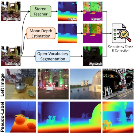
Figure 6: Top: the pseudo-labeling pipeline on in-the-wild internet stereo data. Bottom: visualization of the generated pseudo-labels.
One subtlety matters a great deal: sky regions are excluded from the similarity computation. Sky has infinite depth and is badly underrepresented in the synthetic datasets normally used for training, so including it would corrupt the mask. Sky is detected with open-vocabulary segmentation models, and sky disparity is set to zero in the final pseudo-labels. The remaining disparity maps become the labels, and the consistency mask can optionally select which pixels receive supervision.
Videos are subsampled temporally with a stride of 10, yielding 1.4M usable stereo pairs. The authors stress that comparing in normal space is more robust than comparing directly in depth or disparity space, because normals are locally normalized and therefore insensitive to the wildly varying depth ranges and noisy predictions typical of in-the-wild imagery. This pseudo-labeled data enters the final student training as output-space distillation, complementing the feature-space distillation of the earlier stages.
3. Experiments
3.1 Setup
Fast-FoundationStereo is trained on the same mixed datasets as FoundationStereo plus the pseudo-labeled real data from Sec. 3.4. At deployment time the framework allows free assembly of candidates from each stage into a final model, followed by one end-to-end training run; the resulting fixed weights are then used for zero-shot inference on unseen data. Unless stated otherwise, 8 refinement iterations are used and the maximum disparity for cost volume construction is 192, with no disparity range constraint at evaluation.
Five public datasets are used: Middlebury (indoor pairs with high-quality structured-light ground truth), ETH3D (grayscale pairs, indoor and outdoor), KITTI 2012 and KITTI 2015 (real driving scenes with sparse LIDAR-derived ground truth), and Booster (translucent and specular scenes, targeting non-Lambertian robustness). BP-X reports the percentage of pixels with disparity error larger than X pixels; D1, standard on KITTI, counts pixels whose error exceeds both 3 pixels and 5% of the ground-truth disparity. All results are evaluated on non-occluded regions. Runtime is profiled on an NVIDIA 3090 at Middlebury-Q resolution, which is close to what real-time robotic applications actually use.
3.2 Zero-Shot Generalization
The table below reproduces the core of Table 1 in the paper. Every dataset is unseen by every evaluated method, so this measures pure zero-shot generalization. One fairness measure deserves emphasis: existing real-time methods are not designed for zero-shot generalization and are mostly trained on SceneFlow. For the strong competitors with public training code (RT-IGEV, LightStereo), the authors additionally retrain them on exactly the same data used here, including the proposed pseudo-labels. Those are marked with an asterisk.
| Method | Midd-H BP-2 | Midd-Q BP-2 | ETH3D BP-2 | KITTI-12 BP-2 | KITTI-15 D1 | Runtime (ms) |
|---|---|---|---|---|---|---|
| Not real-time (computationally expensive) | ||||||
| MonSter | - | 4.24 | - | - | - | 336 |
| Zero-RAFT-Stereo | - | 4.68 | - | - | - | 164 |
| FoundationStereo (teacher) | 1.10 | - | - | - | - | 496 |
| Real-time | ||||||
| LightStereo-L (SceneFlow only) | - | 37.21 | - | 14.49 | - | - |
| RT-IGEV* (retrained, same data) | - | 7.82 | - | - | - | 45 |
| Fast-FoundationStereo (ours) | 2.20 | 2.12 | 0.62 | 3.61 | 3.25 | 49 (21) |
Table 1 (excerpt from the paper): zero-shot generalization on public datasets. Full BP-1/BP-3 columns are in the original; the parenthesized runtime is with TensorRT. The proposed method is best in the real-time group in every column, and second-best overall in every column behind the teacher.
Three things stand out. First, the method leads every other real-time model by a wide margin, and it still does so when the competitors are trained on identical data including the pseudo-labels: RT-IGEV retrained reaches 7.82 on Midd-Q BP-2 versus 2.12 here, a factor of 3.7. Second, it matches or beats most of the computationally expensive models, including Zero-RAFT-Stereo, which additionally synthesizes training data with several large foundation models. Third, against the teacher it is more than 10x faster (496 ms down to 49 ms, 21 ms under TensorRT) with only a modest error increase: Midd-H BP-2 moves from 1.10 to 2.20.
Table 2 of the paper isolates non-Lambertian robustness on Booster-Q, with numbers taken from the StereoAnywhere paper. The proposed method reaches BP-2 4.62 and EPE 1.54; the teacher FoundationStereo is 4.07; the strongest real-time competitor RT-IGEV is 16.86, and even its same-data retrained variant is 13.39. On translucent and specular surfaces, the hardest cases in stereo matching, the gap to the teacher (4.62 vs 4.07) is far smaller than the gap to other real-time methods (4.62 vs 13.39). That is good evidence the distillation preserved exactly the priors that are hardest to learn.
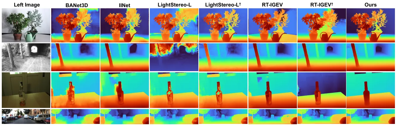
Figure 7: Qualitative zero-shot results of real-time methods on Middlebury, ETH3D, Booster, and KITTI-2015 (top to bottom), with no training on any split of the target datasets. Methods marked with a dagger were trained on exactly the same datasets as ours, including our pseudo-labels.
3.3 Component Ablations
Backbone distillation. Table 3 of the paper compares no distillation (feature backbone pretrained on ImageNet only) against different distillation losses. Distilling the hybrid monocular and stereo priors improves zero-shot generalization broadly, and MSE beats cosine similarity:
| Variant | Midd-H BP-2 | ETH3D BP-1 | KITTI-12 D1 | KITTI-15 D1 |
|---|---|---|---|---|
| No distillation (ImageNet only) | 2.87 | 2.11 | 2.67 | 4.32 |
| Cosine similarity loss | 2.29 | 1.19 | 2.39 | 3.31 |
| MSE loss (ours) | 2.20 | 1.22 | 2.35 | 3.25 |
Table 3 (from the paper): feature backbone distillation ablation. MSE wins on three of four metrics; cosine similarity is marginally better on ETH3D BP-1 (1.19 vs 1.22).
Blockwise search. The blockwise strategy cuts training complexity from $O(n^{N})$ to $O(n)$, but Eq. (1) uses a surrogate objective: it accumulates the impact of perturbing each local block independently, which is only a proxy for the true performance of an assembled candidate. Honest evaluation would require training each full assembled cost filtering module end-to-end with the rest of the network, which is prohibitively expensive. The authors validate the proxy properly. Under the same latency budget $\Delta\tau$, they compare the searched candidate from Eq. (1) against randomly assembled candidates, training all of them end-to-end (remaining parts from the teacher) and evaluating zero-shot, sampling 10 random candidates per $\Delta\tau$. Figure 8 shows three results: as the latency constraint relaxes, the search finds better candidates; across all $\Delta\tau$ values the searched candidate consistently beats random assembly; and as $\Delta\tau$ tightens, some random assemblies degrade substantially, which underscores how much network design matters under a tight budget.
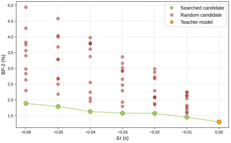
Figure 8: Effects of blockwise architecture search for the cost filtering module under varying latency budget $\Delta\tau$, evaluated on Middlebury-Q. Searched candidates consistently outperform randomly assembled ones.
Pruning ratio. Figure 9 of the paper shows how the pruning ratio affects accuracy on Middlebury-Q and runtime under a single refinement iteration. Aggressive pruning degrades accuracy sharply, and retraining with Eq. (2) recovers it effectively, confirming substantial redundancy in the original refinement module.
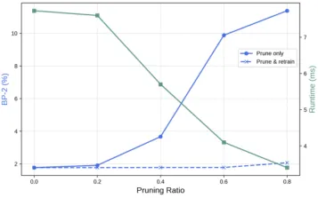
Figure 9: Effects of pruning ratio on accuracy and speed.
Pseudo-labeling. Table 4 of the paper ablates training with and without pseudo-labeled data, and runs the same ablation on several competitive real-time methods. Pseudo-labeling improves generalization consistently for all of them, with much larger gains for methods previously trained only on SceneFlow:
| Method | Midd-H BP-2 | ETH3D BP-1 | KITTI-12 D1 | KITTI-15 D1 |
|---|---|---|---|---|
| RT-IGEV | 11.52 (8.69) | 5.66 (5.12) | 4.54 (3.55) | 6.00 (4.40) |
| LightStereo-L | 23.76 (18.41) | 45.46 (21.12) | 13.98 (5.27) | 12.08 (7.63) |
| Ours | 2.53 (2.20) | 1.31 (1.22) | 2.44 (2.35) | 3.48 (3.25) |
Table 4 (from the paper): results on in-the-wild data without (and with) pseudo-labeling. Parenthesized values are with pseudo-labels; all three methods improve.
The method's own gain from pseudo-labeling is much smaller (BP-2 from 2.53 to 2.20, a 0.33 improvement) than RT-IGEV's (11.52 to 8.69, a 2.83 improvement). That is expected rather than disappointing. The backbone already inherits internet-scale priors through distillation, so the marginal value of additional real data is smaller, whereas RT-IGEV had only ever seen SceneFlow synthetic imagery and benefits enormously from real data. Put differently, distillation and pseudo-labeling both attack the same problem of real-world priors, one from feature space and one from output space, so their returns partially overlap.
3.4 Runtime Decomposition
Figure 10 of the paper breaks down runtime between FoundationStereo and the slowest model in Fig. 2, both profiled on an NVIDIA 3090. Each of the three stages is accelerated by a large margin, summing to an overall speedup above 10x. This decomposition matters because it validates the divide-and-conquer premise itself. If the bottleneck were concentrated in a single stage, compressing the other two would have been wasted effort. In measurement all three stages are bottlenecks of comparable magnitude, which is what justifies hitting each one separately.
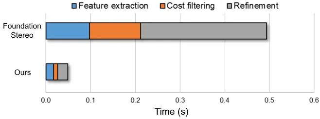
Figure 10: Runtime decomposition. Feature extraction, cost filtering, and disparity refinement are each accelerated substantially, for a total speedup above 10x.
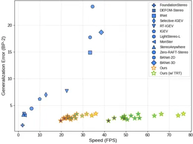
Figure 2: Zero-shot generalization accuracy on Middlebury-Q versus speed for various stereo methods, all measured on the same NVIDIA 3090 GPU. The proposed model family reaches real-time performance with only a slight accuracy decrease relative to the best slow method. Green-outlined stars are further accelerated by TensorRT.
4. Limitations
Quantization is untouched. The authors explicitly list quantization as future work, orthogonal to their distillation, NAS, and pruning, and able to push inference further toward resource-constrained edge devices. That candor leaves a real gap. The reported 49 ms and 21 ms are FP32 and TensorRT graph-optimized numbers; INT8 is never explored. For a method aimed at robot deployment, measurements on edge silicon rather than a desktop 3090 are the numbers that decide usability, and the paper does not provide them.
The ILP objective remains a surrogate. Eq. (1) accumulates per-block perturbations, which implicitly assumes block effects are additive. Cost filtering is a holistic 4D aggregation process, and blocks are plainly coupled: a suboptimal choice at block 3 can shift the input distribution seen by block 5 away from what block 5 was distilled on. The Fig. 8 comparison against random assembly is good evidence that the proxy works, but it establishes that the surrogate beats random selection, not that it recovers the true joint optimum. Finding that optimum requires end-to-end evaluation of each combination, which is precisely what this method avoids in order to escape the $10^{18}$ space.
The gap to the teacher persists on the hardest metrics. Laying the numbers out plainly: Midd-H BP-2 is 1.10 for the teacher and 2.20 here, exactly double, and KITTI-15 D1 is 3.25. The paper's own Table 1 note concedes the method is second-best in every column. On benchmarks already near saturation, a doubled error rate can be a qualitative rather than quantitative change downstream; a manipulator performing close-range grasping with millimeter tolerances is one such case. "Only a slight decrease" is true relative to other real-time methods, but relative to the teacher the concession is substantive.
Pseudo-labels are capped by the teacher. All 1.4M pairs are generated by the teacher model, so in principle the student cannot learn beyond the teacher's competence on this data. Normal-consistency filtering removes the teacher's gross mistakes but not its systematic biases. If the teacher consistently errs on some material, such as a particular reflective coating, that error is written into 1.4M labels and inherited by the student. This is the inherent ceiling of self-distillation.
The three pruning constraints are hand-designed. The constraints in Sec. 2.4 (fixed output channels on the prediction layers, joint pruning of the $h$ pathway, fixed motion-encoder input) are manually written into the dependency graph based on domain understanding of stereo refinement. They are what makes this module prunable, but they also mean the recipe does not transfer for free to other recurrent refinement architectures such as optical flow or scene flow, where the analogous constraints must be re-derived.
5. Takeaways and Outlook
The contribution here is not a new stereo architecture but a reproducible methodology for compressing a slow foundation model into a real-time one. Its central insight is that different parts of a foundation model bottleneck for different reasons and therefore deserve different tools. Feature extraction is expensive because of the ViT backbone, so use architecture-agnostic distillation into a mature lightweight CNN. Cost filtering is expensive because of 4D attention, its channels are already too thin to prune, and humans cannot design good replacements, so hand it to NAS. Refinement is expensive because of recurrent redundancy, so use structured pruning with retraining. Three targeted strikes, then a unified assembly and end-to-end training pass.
The most transferable piece is the blockwise search. A space of $200^{8}\approx10^{18}$ combinations is hopeless by brute force, and the authors turn an exponential problem into a linear one ($O(n^{N})\to O(n)$) through independent per-block distillation, independent per-block evaluation, and ILP combination, then verify the surrogate objective against randomly assembled candidates. The recipe is not specific to stereo. Any deep network that can be cut into serial blocks with fixed interfaces admits the same divide-and-conquer search.
The normal-consistency check in the pseudo-labeling pipeline is the second idea worth carrying away. Using a monocular depth estimator and the stereo teacher as mutual cross-validation, converting both outputs into normal maps, and comparing cosine similarity works because normals are locally normalized and thus robust to the extreme depth ranges and noisy predictions of in-the-wild imagery, far more so than comparing directly in depth or disparity space. This pattern of geometric consistency as automatic quality control applies to essentially any self-labeling or pseudo-labeling curation pipeline.
Looking forward, the authors point to quantization. The broader question is how far this methodology generalizes. This paper addresses stereo matching, but the entire embodied-AI field faces the same bind: many powerful foundation models (VLA policies, world models, diffusion policies) are excluded from robot bodies by inference latency. Divide-and-conquer compression, blockwise NAS, and teacher-bootstrapped pseudo-labels on real data are all plausibly portable to those settings. If they are, the current assumption that foundation models are too slow and must live in the cloud may loosen considerably.
6. Lines Worth Remembering
"Each of these steps is accelerated by a divide-and-conquer strategy." The sentence the whole paper hangs on: three stages, three different bottlenecks, three different tools, not one hammer.
"Direct pruning of the cost filtering modules yields severe performance degradation for only marginal speedup, since the channel dimension in $\mathbf{V_{C}}$ is already small (mostly under 100)." A very specific negative result that explains why this stage had to go to NAS.
"Our blockwise distillation reduces training complexity from $O(n^{N})$ to $O(n)$." Exponential to linear: the hardest engineering result in the paper.
"In contrast to directly comparing in the depth or disparity space, our proposed normal consistency check is more robust to extremely diverse depth ranges or noisy predictions on in-the-wild images." The design point of the pseudo-labeling pipeline, and a directly reusable trick.
"Exploring quantization techniques offers an orthogonal avenue to further enhance inference speed." The authors flagging their own next step, and a hint that 49 ms and 21 ms are not the floor for this approach.