PAPER DEEP DIVE
Efficient On-policy Visual-RL via Stochastic Decoupled Policy Gradient
We present the stochastic decoupled policy gradient (SDPG), a lightweight visual reinforcement learning (RL) method that trains diverse visuomotor control policies end-to-end within a few hours on a single NVIDIA RTX 4080 GPU. SDPG estimates policy gradients via random perturbations of trajectory rollouts, requiring orders of magnitude fewer batch-rendered environments and substantially reducing compute and memory overhead. On visual MuJoCo benchmarks, SDPG consistently outperforms baseline methods in training time, memory usage, and rewards. Finally, to support future research, we introduce a suite of realistic visual robotics benchmarks spanning dexterous manipulation, challenging locomotion, and demonstrate effective sim-to-real transfer on physical hardware.
Paper Information
Title: Efficient On-policy Visual-RL via Stochastic Decoupled Policy Gradient.
Authors: Haoxiang You, Yilang Liu, Davis Zong, Qian Wang, Teeratham Vitchutripop, Qi Wang, Daniel Rakita, and Ian Abraham.
Links: arXiv 2605.26478, the official repository at HaoxiangYou/SDPG, and the project website. The repository is MIT-licensed and describes itself as the official implementation. It provides training, evaluation, replay, baseline configurations, and both state- and vision-based task settings.
One-Sentence Summary
SDPG turns policy improvement into a return-difference estimate over random action perturbations around shared nominal states, so only a small set of environments needs camera rendering while many physics-only environments estimate the update direction.
Background And Motivation
Learning visuomotor control directly from images is attractive because deployed robots receive cameras, proprioception, and sometimes depth rather than simulator state. The learning system must simultaneously build visual representations, assign credit over long horizons, and search in a continuous action space. SDPG does not propose a new transformer or a new simulator. Its central claim is architectural: the compute spent on visual RL can be reorganized so that high-quality policy-gradient search no longer requires thousands of rendered environments.
The paper contrasts three existing routes. Off-policy visual methods such as DrQ-v2 and model-based systems such as DreamerV3 learn strong policies but require many sequential gradient updates. In wall-clock terms, image augmentation, world-model training, replay sampling, and representation updates remain expensive. On-policy methods such as PPO are easier to reason about but reduce gradient noise by collecting from very large batches. When every environment emits RGB, the rendering buffer dominates memory.
Teacher-student distillation is the most common robot-learning workaround. A teacher sees privileged state, and a visual student imitates it with DAgger. This pipeline is fast and often deployment-friendly, but the authors identify two structural failure modes. The student lacks privileged information, creating information asymmetry. More importantly, the student makes mistakes that carry it into states absent from the teacher's supervision distribution. Once the robot is falling, twisted, or outside the trained local manifold, another imitation loss cannot recover a useful action.
Differentiable simulation offers another route: backpropagate through physics into actions and then into policy parameters. This yields low-variance first-order gradients, but it couples learning to differentiable contact, rendering, and reward implementations. Long contact chains can explode or vanish, soft contact models may drift from production simulators, and many useful robotics rewards or sensor models are not cleanly differentiable.
SDPG targets this gap. It keeps the on-policy structure and the idea that return differences reveal better actions, but it avoids analytical trajectory Jacobians. It also avoids rendering every perturbed trajectory. The resulting algorithm behaves like policy gradient in its data discipline, yet allocates rendering only where the policy must learn perception.
Preliminaries
The dynamical system is $\mathbf{s}_{t+1}=f(\mathbf{s}_{t},\mathbf{a}_{t})$, observations are produced by $\mathbf{o}_{t}=g(\mathbf{s}_{t})$, and a parameterized policy maps observations to continuous action distributions. The optimization objective is the expected discounted return over initial states:
$$\boldsymbol{\theta}^{\star}=\arg\max_{\boldsymbol{\theta}}\mathcal{V}(\boldsymbol{\theta})\coloneqq\mathbb{E}_{\mathbf{s}_{0}\sim\rho_{0}}\big[\mathcal{J}(\mathbf{s}_{0},\boldsymbol{\theta})\big].$$
Here $\boldsymbol{\theta}$ denotes actor parameters, $\rho_{0}$ is the initial-state distribution, and $\mathcal{J}$ is a trajectory return. Conventional first-order RL differentiates through the trajectory:
$$\nabla_{\boldsymbol{\theta}}\mathcal{V}=\mathbb{E}_{\tau}\Big[\frac{d\mathbf{A}}{d\boldsymbol{\theta}}^{\top}\nabla_{\mathbf{A}}\mathcal{J}\Big].$$
The action sequence $\mathbf{A}$ depends on state dynamics, observations, and the policy. The total derivative $d\mathbf{A}/d\boldsymbol{\theta}$ therefore contains the expensive feedback path through future states. Prior decoupled policy gradients stop gradient through observations and replace the total derivative with a partial derivative. SDPG goes one step further by replacing the analytical action-sequence gradient itself with a stochastic smoothing estimate.
Method
Smoothed Gradient Estimation
For a nominal action sequence $\mathbf{A}$, SDPG samples $M$ Gaussian action-sequence perturbations $\mathcal{E}^{j}$. Each perturbation is executed from the same physical state as the corresponding nominal environment. The return difference is multiplied by the noise vector and normalized:
$$\nabla\mathcal{J}_{\text{smooth}}(\mathbf{A})\coloneqq\mathbb{E}_{\mathcal{E}\sim\mathcal{N}(\mathbf{0},\mathbf{I})}\Big[\frac{\mathcal{J}(\mathbf{A}+\delta\mathcal{E})-\mathcal{J}(\mathbf{A})}{\sigma}\mathcal{E}\Big]\approx\frac{1}{M}\sum_{j=1}^{M}\Big(\frac{\mathcal{J}(\mathbf{A}+\delta\mathcal{E}^{j})-\mathcal{J}(\mathbf{A})}{\sigma}\mathcal{E}^{j}\Big).$$
The vector $\delta$ is the exploration scale and $\sigma$ is the standard deviation of return differences. Theorem 1 states that this estimator is proportional to the gradient of the Gaussian-smoothed objective $\mathcal{J}_{\delta}(\mathbf{A})=\mathbb{E}_{\mathcal{E}}[\mathcal{J}(\mathbf{A}+\delta\mathcal{E})]$. Thus SDPG is not abandoning gradients for blind search. It is choosing which derivative is safe and cheap to estimate.
The replacement has three practical consequences. First, dividing by $\sigma$ prevents returns with a different scale from producing pathological steps. Figure 3 shows large policy-gradient-norm spikes for SAPO on Allegro Hand, while SDPG remains in a much lower band. Second, only forward simulation and returns are required; contact, rewards, and sensors need not be differentiable. Third, the resulting direction can be consumed by a supervised policy objective, so no backward pass crosses rendering or physics.
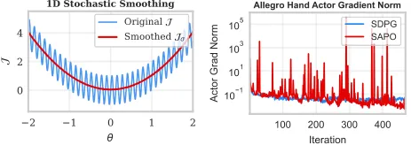
Figure 3: A one-dimensional smoothed objective and the gradient-norm comparison between SDPG and SAPO.
From Search Direction To Backpropagation
Proposition 1 converts an explicit action-space ascent step into a regression objective. If $\mathbf{d}(\mathbf{A}_{k})$ is the desired update direction, define a stop-gradient target one step ahead:
$$\boldsymbol{\theta}_{k+1}\leftarrow\boldsymbol{\theta}_{k}-\beta\nabla_{\boldsymbol{\theta}_{k}}\mathcal{L},\quad\mathcal{L}\coloneqq\tfrac{1}{2}\|\mathbf{A}_{k}-\mathbf{A}_{k}^{\mathrm{target}}\|^{2},\quad\mathbf{A}_{k}^{\mathrm{target}}\coloneqq\mathrm{sg}\big(\mathbf{A}_{k}+\mathbf{d}(\mathbf{A}_{k})\big).$$
Differentiating the loss through the predicted action gives exactly the partial Jacobian multiplied by the negative update direction. The stop gradient prevents the target from being treated as a differentiable function of current parameters. The SDPG actor objective is therefore:
$$\mathcal{L}(\boldsymbol{\theta},\mathbf{O},\mathbf{A})\coloneqq\mathbb{E}\left[\|\pi(\mathbf{O}\mid\boldsymbol{\theta})-\mathrm{sg}\big(\mathbf{A}+\nabla\mathcal{J}_{\text{smooth}}(\mathbf{A})\big)\|_{2}^{2}\right].$$
The equivalent policy improvement direction is:
$$\nabla_{\boldsymbol{\theta}}\mathcal{V}_{\text{SDPG}}\approx\mathbb{E}_{\tau,\mathbf{s}_{0}}\Big[\frac{1}{M}\sum_{j=1}^{M}\frac{\partial\mathbf{A}}{\partial\boldsymbol{\theta}}^{\top}\frac{\mathcal{J}(\mathbf{A}+\delta\mathcal{E}^{j})-\mathcal{J}(\mathbf{A})}{\sigma}\mathcal{E}^{j}\Big].$$
Only the actor receives gradients. Rendering and state transitions do not. The visual encoder learns because it must predict actions that produced higher local returns, not because a synthetic camera model is differentiable. This preserves ordinary vision architectures while retaining an improvement signal.
A Unified View Of Policy Gradient Methods
The paper makes the relation to ordinary policy gradient explicit. For a Gaussian policy $\mathbf{u}_{t}=\mathbf{a}_{t}+\delta\boldsymbol{\epsilon}_{t}$, using the mean-action return $\mathcal{J}(\mathbf{A})$ as the baseline gives:
$$\nabla_{\boldsymbol{\theta}}\mathcal{V}_{\text{PG}}=\mathbb{E}_{\tau,\mathbf{s}_{0}}\Big[\frac{\partial\mathbf{A}}{\partial\boldsymbol{\theta}}^{\top}\frac{\mathcal{J}(\mathbf{A}+\delta\mathcal{E})-\mathcal{J}(\mathbf{A})}{\delta}\mathcal{E}\Big].$$
Classical policy gradient is therefore the $M=1$ special case with $\delta$ in the denominator. SDPG averages $M$ perturbations and normalizes by the return-difference scale $\sigma$. That small algebraic change has a large systems implication. To reduce variance, ordinary policy gradient increases the number of rendered nominal trajectories. SDPG increases physics-only perturbations around each nominal trajectory, while visual processing remains tied to the nominal set.
The authors also reinterpret policy learning as guided search. A target action sequence can be formed by local trajectory optimization, followed by a weighted behavior-cloning update. They prove that decoupled policy gradient is exactly one trajectory-search step plus one policy regression step. Classical guided policy search performs multiple search and distillation iterations per batch. SDPG performs stochastic search once and then regresses the policy, placing it on the policy-gradient side of the same continuum.
This perspective matters for tuning. Search-related choices, such as horizon, exploration scale, and perturbation count, can first be studied with low-dimensional state observations. Then the same search configuration can be transferred to a visual policy by adding an encoder. The paper reports that this transfer preserves final reward while vision usually requires two to four times more iterations for representation learning.
Nominal And Physics-Only Environments
Each iteration uses $N$ nominal environments with batch rendering and $M$ state-only auxiliary environments for each nominal trajectory. The default benchmark configuration uses $N=64$ and $M=63$, yielding 4096 physical environments but only 64 rendered environments. At the start of every short rollout segment, each auxiliary environment copies the exact internal state of its nominal environment.
Reset handling preserves the comparison. If an auxiliary environment terminates, it is reset to the current state of its nominal environment. If the nominal environment terminates, all of its auxiliaries reset together. Consequently, return differences compare actions from the same origin and the same surviving prefix, rather than mixing unrelated initial conditions.
The official implementation exposes this structure directly. In agents/sdpg.py, rollout() computes mean actions once for the nominal observations, broadcasts the mean and exploration scale, and samples noise only for auxiliary rows:
out = self.actor(actor_obs)
nominal_actions = out["mean"].repeat_interleave(self.num_action_perturbations + 1, dim=0)
eps_actions = torch.randn_like(nominal_actions)
eps_actions[self.nominal_env_ids] = 0.0
actions = nominal_actions + eps_actions * std
obs, rewards, terminated, truncated, info = self.env.step(torch.tanh(actions), auto_reset=False)
This corresponds to agents/sdpg.py:409-433. Nominal indices are constructed at agents/sdpg.py:40-42. Auxiliary-to-nominal index mapping is implemented at agents/sdpg.py:765-803, and state-copy reset behavior is implemented at agents/sdpg.py:805-835. Together these code paths match the short-horizon rollout diagram in Figure 6.
Short Horizons, Critic, And Exploration
SDPG does not differentiate through an arbitrarily long episode. It uses short rollout segments and bootstraps the tail with a learned value:
$$\mathcal{J}=\sum_{t=0}^{H}\gamma^{t}r_{t}+\gamma^{H+1}V_{\phi}(\mathbf{s}_{H+1}).$$
The critic consumes privileged low-dimensional state, while the actor consumes deployable observations. The value function is trained with standard TD targets, and a target critic tracks the online critic slowly. This split accelerates credit assignment without introducing a privileged input at deployment time.
The exploration factor is also learned. Let $\tilde{\delta}=\log\delta$. The paper derives a stop-gradient target from the return curvature induced by action noise:
$$\mathcal{L}_{\tilde{\delta}}\coloneqq\mathbb{E}\Big[\|\tilde{\delta}-\mathrm{sg}(\tilde{\delta}^{\text{target}})\|_{2}^{2}\Big],\quad\tilde{\delta}^{\text{target}}\coloneq\tilde{\delta}+\frac{\mathbf{I}}{T}\mathbb{E}_{\mathcal{E}}\Big[\frac{\delta}{\sigma}\big(\mathcal{J}(\mathbf{A}+\delta\mathcal{E})-\mathcal{J}(\mathbf{A})\big)(\mathcal{E}^{2}-1)\Big].$$
If larger exploration improves expected return, the target increases $\delta$; if long steps damage return, it shrinks. The implementation can combine this update with actor entropy regularization and a target standard deviation. The appendix recommends state-independent exploration plus actor entropy regularization as the simplest configuration that transfers across tasks.
In the source, compute_delta_J() supports noncausal return differences, causal return-to-go, and TD eligibility traces. compute_ascent_direction() groups rewards and noise by nominal environment, computes per-timestep variance, optionally normalizes $\Delta\mathcal{J}$, and averages the weighted noise:
delta_J = self.delta_J.view(self.num_base_envs, self.num_action_perturbations + 1, self.horizon_length)
delta_J_var = delta_J.var(dim=1)
if self.normalize_delta_J:
    delta_J = delta_J / (torch.sqrt(delta_J_var).unsqueeze(1) + 1e-6)
mean_weighted_grouped = delta_J.unsqueeze(-1) * eps
mean_ascent_direction = mean_weighted_grouped.mean(dim=1)
This code corresponds to agents/sdpg.py:584-637. At agents/sdpg.py:645-693, train_actor() adds the ascent direction to nominal actions, treats the result as a stop-gradient target, and minimizes MSE over both mean and log standard deviation. Critic regression and target-network soft updates are at agents/sdpg.py:695-742. The implementation is therefore a direct operationalization of Equations 1, 3, and 10.
flowchart TB
    N["64 nominal envs batch rendering"] --> A["actor mean actions"]
    A --> P["63 physics-only perturbations per nominal env"]
    N --> R["nominal return baseline"]
    P --> D["perturbed returns"]
    R --> D
    D --> G["Delta J weighted noise direction"]
    G --> T["stop-gradient action targets"]
    T --> U["actor MSE update"]
    P --> C["privileged-state TD lambda critic"]
    C --> B["bootstrap short rollout"]
    B --> D
    A --> S["learn exploration factor"]
    G --> S
SDPG execution and update flow: rendering is restricted to nominal environments, while return differences come from matched physical perturbations.
Implementation Anatomy
The runner mirrors the paper in a way that is useful to inspect before reusing the code. During initialization, it records the number of nominal environments and the number of action perturbations separately, then computes the flat environment index for every nominal row. The repository's comments make the layout explicit: a nominal environment is followed by its auxiliary rows, and a training invocation with the default settings creates 64 groups of 64 environments. This is why the same simulation backend can maintain 4096 copies of the physics scene while the actor image batch remains based on 64 observations.
The actor and critic are separate modules rather than one shared network with two heads. The actor takes its configured deployable inputs, runs one encoder per input source, concatenates the encoded features, and passes them to an MLP policy head. The critic can consume privileged observations or extra height fields that the actor never sees. This is not merely a convenience; it preserves the paper's distinction between the controlled information available to a real robot and the denser signals useful for a learned value function in simulation.
Action generation is also close to the equations. The actor returns a mean and log standard deviation. The runner repeats both across the nominal-plus-auxiliary group, clips mean actions and log standard deviations when bounds are configured, samples standard normal noise, zeroes the noise on nominal rows, and constructs perturbed actions as the mean plus scaled noise. The environment receives a hyperbolic tangent of the raw action, so the bounded control convention is consistent between nominal and auxiliary environments.
Return differences are not a single hardcoded estimator. The repository can assign a segment-level return difference to every step, compute a causal return-to-go difference at every time index, or apply an eligibility-trace formulation. This matters for robotics tasks with different time constants. A short contact-rich manipulation segment may benefit from causal credit, while a terrain locomotion rollout may prefer the simpler configuration used for Go2Terrain.
Normalization is another place where the implementation adds engineering detail. The code computes the variance of $\Delta\mathcal{J}$ across the perturbation dimension for each nominal environment and timestep, then divides by its square root with a small epsilon when normalization is enabled. This is the practical counterpart of replacing the fixed exploration scale in the denominator of ordinary policy gradient with the empirical return scale used by SDPG.
The actor update creates stop-gradient targets from the nominal actions plus the averaged weighted noise. It regresses both the action mean and the learned log standard deviation, applies optional entropy regularization, clips gradients, and performs one optimizer step. A separate temperature optimizer can tune the entropy coefficient toward a target policy standard deviation. In several vision configurations the entropy block is intentionally disabled; the code keeps that as an explicit task decision rather than baking one exploration heuristic into every benchmark.
The critic update uses more data than the actor. By default it can use nominal and auxiliary transitions to train the value function, shuffles the flattened dataset, draws large mini-batches, performs multiple critic iterations, and then soft-updates a target critic. This asymmetry is coherent: the actor must remain tied to one fresh policy-gradient sample set, while the critic is a bootstrap device and can profit from every matched perturbation without needing rendered images.
Configuration files expose the task-specific decisions in readable form. State tasks use pass-through privileged observations, while visual tasks add DrQ-v2-style RGB encoders or depth encoders. Manipulation configs often shorten the horizon and tighten gradient clipping; humanoid and quadruped configs change target-critic coefficients, reward scaling, learning-rate schedules, and exploration settings. The default 64-by-63 grouping stays stable across many tasks, which supports the authors' claim that search-related structure can transfer even when representation and control details change.
Evaluation and replay are also part of the release rather than afterthoughts. A trained checkpoint can be loaded with the same task and agent configuration used during training, evaluated headlessly on a remote machine, and replayed locally from the saved trajectory. This workflow is important for robotics because debugging a failed policy often requires separating policy error from renderer, physics, state reset, or deployment latency; replaying the simulator trajectory makes those failures inspectable.
The repository's current scope should be read accurately. It supports Genesis-based environments and includes vendored baselines, but sections for other simulation backends and hardware integration are marked as coming soon in the README. Thus the strongest reproducibility today is in the algorithm, MuJoCo-compatible environments, ego-centric suite, and training pipeline, not in turnkey support for every robot platform.
That implementation shape also explains why the method is attractive for small labs. The expensive resource is no longer thousands of simultaneous camera buffers; it is the physics solver and a modest set of rendered observations. A researcher with one 16 GB GPU can reproduce search behavior at scale, study exploration, and test reward shaping before renting a cluster or falling back to privileged teacher distillation.
Reading The Results Carefully
The benchmark comparison is strongest when read as a systems result rather than a single number. SDPG does not claim to dominate every off-policy method on every axis. Instead, it shows that a policy-gradient family usually excluded from large-scale visual control can reach competitive reward while staying within the memory envelope of off-policy and model-based baselines. The training-time advantage comes from fewer rendered environments and no trajectory backward pass, not from magically reducing simulation steps.
The distillation comparison has a similar nuance. The state teacher remains an excellent tool and can be faster on moderately difficult tasks. The paper's useful observation is where the teacher-student assumption breaks: when the student enters falling or contorted states that the teacher never visited, direct visual RL can keep collecting informative failures. This makes SDPG especially relevant for humanoid and contact-rich tasks where failure boundaries are close to the operating envelope.
The two-to-four-times iteration gap between state and vision inputs is also valuable. It says that adding perception does not necessarily require retuning the entire local search procedure. The CNN needs more updates to learn a representation, but exploration scale, perturbation count, and horizon can often be transferred from state experiments. For practitioners, that turns a costly visual sweep into a cheaper state sweep followed by a focused representation check.
Finally, the benchmark suite broadens the evidence beyond classic continuous-control environments. The ego-centric tasks include multi-camera manipulation, in-hand reorientation, humanoid hurdling, and depth-based terrain traversal. They are not merely visual wrappers around state tasks: actor inputs mimic onboard sensing, while critic inputs may retain privileged terrain and state information. That division is consistent with the method's goal of training deployable perception policies without pretending that all learning signals must be deployable.
Experiments
The MuJoCo benchmark is reimplemented in Genesis. Hopper, Walker, Ant, and Humanoid actors receive third-person RGB images, while critics use privileged state. All visual baselines run on one NVIDIA RTX 4080. DrQ-v2 and DreamerV3 receive parallel-simulation and code optimizations for fair wall-clock comparison. The distillation baseline follows recent practice: train a state teacher with RL-games or RSL-RL PPO, then train a visual student.
The training curves in Figure 8 show that SDPG matches state-based teacher performance on the benchmark suite. Teacher-student distillation is competitive on the easier Hopper and Walker settings, but on Ant and especially Humanoid the visual student tends to plateau or enter unstable states. SDPG continues improving while remaining on-policy and end-to-end. The authors do not claim distillation is universally worse; they identify task difficulty and student-state coverage as the decisive factors.
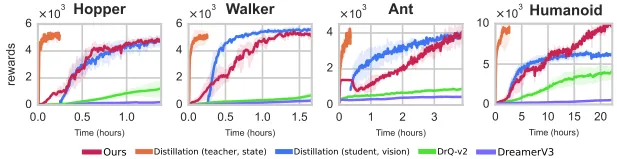
Figure 8: Wall-clock reward curves for SDPG, distillation, DrQ-v2, and DreamerV3 on visual MuJoCo.
Memory is the clearest quantitative result. With 64 batch-rendered environments, SDPG uses 10.2 to 10.5 GB across the four tasks. The PPO estimate with 4096 environments and state-based hyperparameters rises to roughly 48 to 50 GB. DrQ-v2, DreamerV3, and distillation remain in a similar single-GPU range, but their learning dynamics and sample reuse differ. The important result is that an on-policy end-to-end visual method now fits the same memory budget without clustering.
| Method | Hopper | Walker | Ant | Humanoid |
|---|---|---|---|---|
| SDPG | 10.2 GB | 10.3 GB | 10.3 GB | 10.5 GB |
| PPO estimated | 48 GB | 48 GB | 49 GB | 50 GB |
| DrQ-v2 | 10.6 GB | 8.2 GB | 10.5 GB | 11.6 GB |
| DreamerV3 | 10.8 GB | 10.8 GB | 10.8 GB | 10.9 GB |
| Distillation | 10.6 GB | 10.6 GB | 10.3 GB | 10.7 GB |
Table 1: Visual MuJoCo memory usage. PPO is estimated with 4096 environments and state-based hyperparameters; other methods use 64 batch-rendered environments.
Figure 9 adds a qualitative check that average reward alone can hide. In humanoid rollouts, the vision-distilled student can fall or lose a stable gait in particular states, whereas SDPG maintains running and recovery. The observation is consistent with the paper's broader argument: once the visual policy enters underrepresented states, supervision from a teacher with different observations is not enough; collecting consequences in the current policy distribution helps.
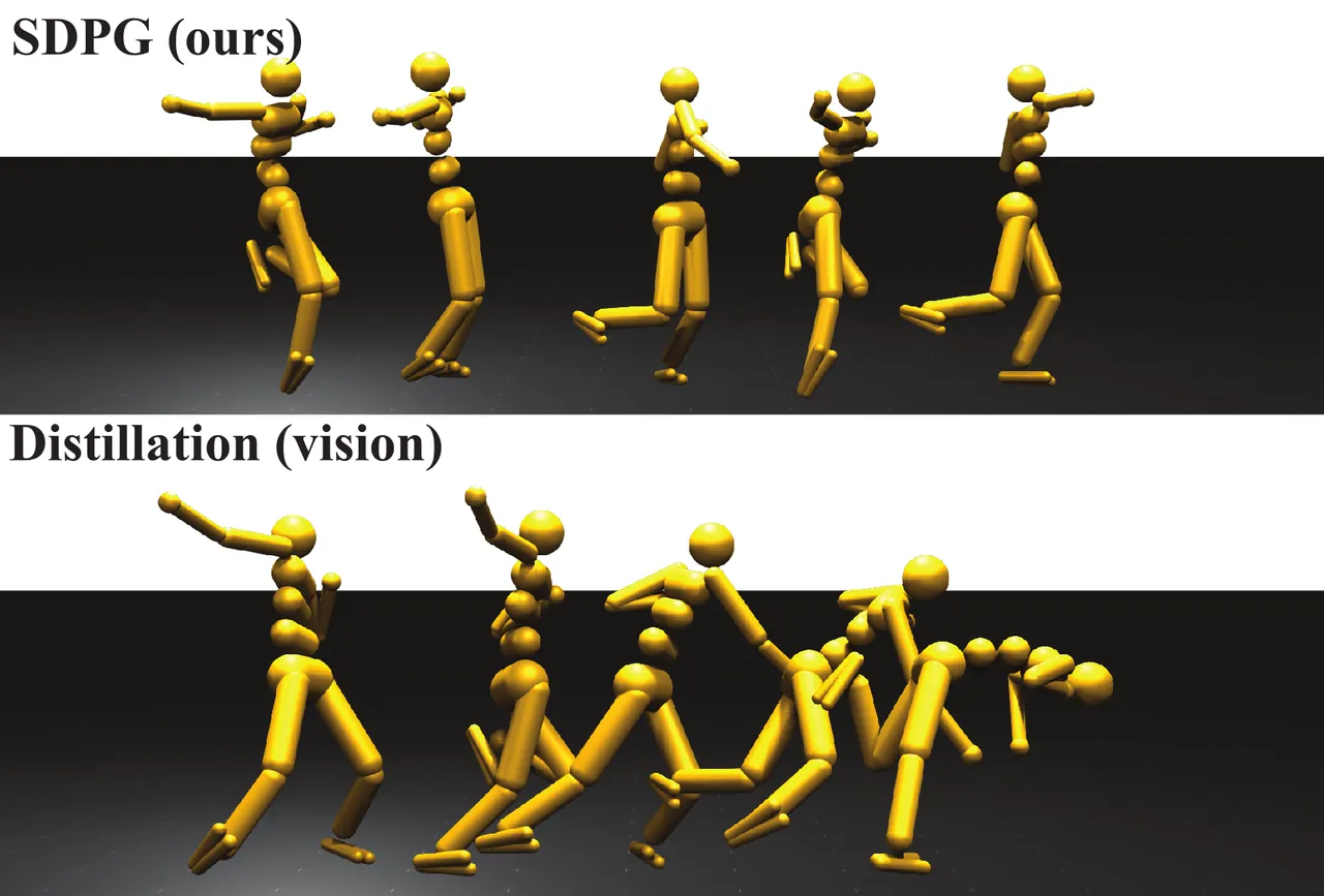
Figure 9: Humanoid trajectory comparison between SDPG and a visual distillation policy.
The state-versus-vision experiment supports the guided-search interpretation. The authors tune trajectory-search hyperparameters with state observations and then reuse them for visual training with only a CNN encoder added. Final rewards are similar, while visual learning requires two to four times more iterations. This separation is useful in practice because search and representation failures then produce different symptoms and can be debugged separately.
Beyond MuJoCo, the paper introduces an ego-centric suite designed for realistic robot sensing. The actor combines proprioception with one or more ego-centric cameras. The tasks cover locomotion, manipulation, dexterous hands, RGB and depth input, single- and multi-camera settings, and terrain variation.
| Environment | Robot and task | Visual modality | Actor cameras |
|---|---|---|---|
| WalkerHurtle | Planar walker jumps over hurdles | RGB or depth | 1 |
| G1Hurtle | Unitree G1 humanoid jumps over hurdles | RGB or depth | 1 |
| Go2Terrain | Unitree Go2 traverses procedural terrain | RGB or depth | 1 |
| FrankaPickCube | Franka Panda picks a cube | RGB | 1 |
| AlohaInsertion | Bimanual ALOHA performs peg insertion | RGB | 3 |
| AllegroHand | In-hand cube reorientation | RGB | 1 |
| ShadowHand | In-hand cube reorientation | RGB | 1 |
Table 2: The ego-centric benchmark suite spans humanoid and quadruped locomotion, arm manipulation, bimanual insertion, and in-hand reorientation.
The configurations reveal how the method is adapted across contact scales. Most tasks retain $N=64$ and $M=63$. Rollout horizons vary from 16 to 64 steps. Go2Terrain uniquely uses a ten-times reward scale and disables both causality and eligibility traces. AlohaInsertion reduces nominal trajectories to 48 because four image encoders do not fit at the default setting. These choices show that SDPG is not a single fixed recipe, although its core resource split remains unchanged.
| Hyperparameter | Paper default | Role |
|---|---|---|
| Nominal environments $N$ | 64 | Sets the number of batch-rendered environments |
| Auxiliary environments per nominal $M$ | 63 | Sets the number of perturbation samples |
| Total physical environments | 4096 | Equal to $N(M+1)$ |
| Discount factor $\gamma$ | 0.99 | Shared long-horizon return weighting |
| TD coefficient | 0.95 | Blends multi-step return-to-go estimates |
| Critic mini-batch | 4096 | Uses a large sample pool for stable value regression |
| Actor updates per epoch | 1 | Keeps the one-step policy-gradient structure |
Table 3: Key training settings shared across most environments.
The hardware experiment tests whether this training structure survives the sim-to-real boundary. A Unitree Go2 uses an ego-centric RealSense depth camera and proprioception. The policy is trained entirely in simulation for about two hours and deployed zero-shot on stairs, boxes, large stones, and downhill terrain. The reported transfer is not fine-tuned on hardware, so it provides evidence that the depth, control, and domain-randomization pipeline covers the selected terrain family.
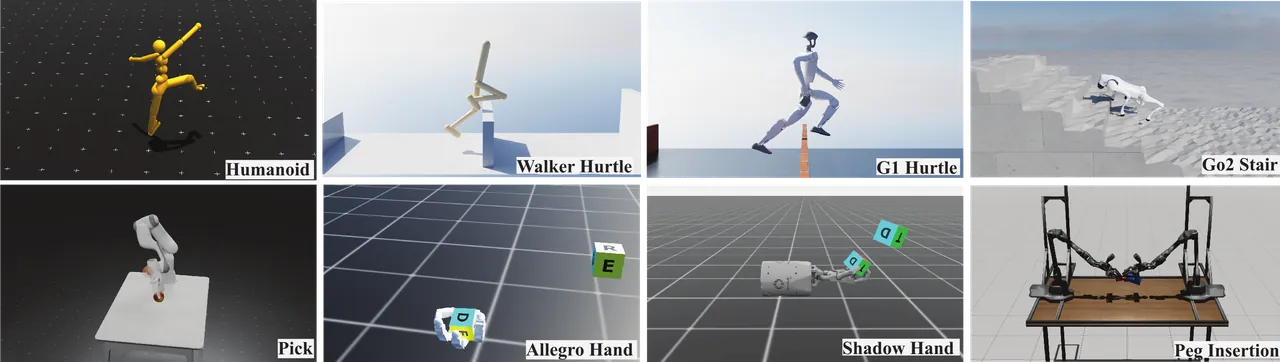
Figure 2: The suite covers humanoid and quadruped locomotion, manipulation, dexterous hands, and third-person or ego-centric sensing.
Limitations
The authors are explicit about two constraints. Although memory is modest, total compute remains dominated by physics rollouts. Samples are discarded after each iteration, making SDPG closer to early A2C than to PPO with multiple reuse epochs. The authors also report sensitivity to random seeds and occasional instability, and they identify PPO-style stabilization and sample reuse as future work.
The memory advantage depends on a simulator's ability to copy exact internal state into many auxiliary environments. This is natural in Genesis for the tested rigid-body tasks, but may be harder when sensor state, fluid, deformation, latency, or external hardware state must be replicated. If auxiliary-state copying becomes expensive or approximate, increasing $M$ no longer remains cheap.
The derivation is centered on Gaussian exploration and continuous control. Discrete decisions, multimodal behavior, and information-gathering tasks may need a different target parameterization. The authors note that their autoregressive action-regression form avoids likelihood ratios and could later support diffusion actors, but the current implementation uses MLP and CNN policy heads rather than such high-capacity sequence models.
Finally, the wall-clock and memory numbers are tied to Genesis, its rendering backend, and an RTX 4080. The authors did optimize DrQ-v2 and DreamerV3, but PPO memory remains an estimate rather than a directly measured run under the identical visual configuration. Cross-simulator adoption should therefore begin with a small reproduction before extrapolating the reported speedup.
Conclusion
SDPG's contribution is precise rather than mystical. Ordinary policy gradient is the $M=1$ case with $\delta$ as denominator. SDPG averages many matched perturbations and uses the return-difference standard deviation for numerical stability. That change makes random action exploration a useful local search signal while preserving the one-update-per-rollout discipline of policy gradient.
For robot-learning practitioners, the paper offers a practical single-GPU recipe: render only nominal visual observations, use privileged state for the critic, put physics-only perturbations around each nominal state, and use short bootstrap horizons. On tasks expressible in Genesis, this is a credible first alternative to large-batch visual PPO or teacher-student distillation.
For engineers porting the repository to a new robot, the important questions are not only learning rates. Check whether simulator state can be copied exactly, whether simulated depth or RGB latency matches deployment, and whether rollout length and exploration scale match the robot's controllable time constants. Those choices determine whether the matched-perturbation signal remains a valid improvement direction.
A useful adoption path is therefore incremental. Reproduce one state task, then one visual benchmark, then run the same checkpoint through replay and hardware-in-the-loop checks before attempting a new platform. This preserves the paper's matched-state assumption and makes the source of any real-world failure easier to isolate.
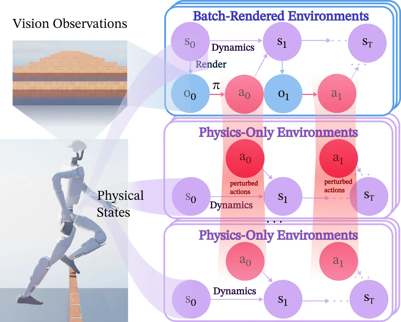
Figure 1: Batch-rendered environments produce visual actions, while physics-only environments evaluate perturbed actions from matched states.
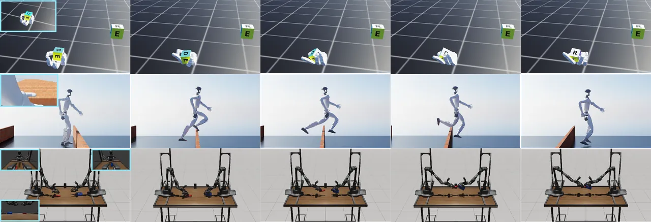
Figure 4: Visual environments scale poorly in memory, so SDPG confines rendering to the nominal environment set.
Golden Quote
Do not render four thousand camera views to reduce gradient noise. Reserve rendering for a few nominal states and let cheap state physics carry the perturbations.