SGM-SLAM: Scene Graph Matching for Data-Efficient Distributed SLAM

Authors: Yewei Huang, Tixiao Shan, Abhinav Rajvanshi, Niluthpol Chowdhury Mithun, Yaxuan Li, Brendan Englot, and Han-Pang Chiu · Paper: arXiv:2606.16881 · Code status: no public implementation is provided in the paper, and repository searches did not find a same-named release.

Background and Motivation

Multi-robot SLAM becomes difficult at the boundary between two local maps. Each robot can estimate its own trajectory with LiDAR-inertial odometry, but that trajectory is expressed in a frame initialized at its own starting pose. Without GPS or a central coordinator, the team must discover which observations describe the same physical objects and estimate the transformation between independently initialized world frames. This data-association step determines whether the resulting map is coherent: a wrong inter-robot loop can pull trajectories into a distorted alignment, while a missed loop can leave otherwise accurate local maps permanently disconnected.

Feature-level methods approach this by comparing appearance or scan geometry. Visual bag-of-words descriptors are sensitive to illumination and viewpoint. LiDAR descriptors such as Scan Context are compact, but they require enough overlap between scans to form a stable signature. The paper's experiments expose both failure modes. In the outdoor sequence, where two trajectories have little overlap, a Swarm-SLAM configuration using Scan Context produced 20.29 m absolute trajectory error. Indoors, weak lighting and a height difference between a handheld rig and a quadruped platform made a CosPlace image descriptor less reliable; that configuration reached 5.70 m error. These are not merely implementation failures. They show that the representation used for candidate generation must survive the exact conditions in which rendezvous evidence is scarce.

Scene graphs offer a different organization. Instead of treating the map as an undifferentiated point cloud, a scene graph retains objects, keyframes, semantic point clouds, and relations among them. This structure is easier to query for task planning and easier for people to interpret. It can also carry localization evidence. Hydra, Hydra-multi, and Kimera-Multi demonstrated the value of 3D scene graphs, but many systems either match scene graphs with visual descriptors or centralize map fusion. In a low-bandwidth outdoor deployment, both choices can delay updates or overload the network.

The authors narrow the problem to a useful observation: before two robots exchange point clouds, they do not need a complete map or a high-dimensional descriptor. If each robot can extract discrete objects from fused RGB-LiDAR data, the tuple of object class, centroid, and inter-object distance already has enough structure for matching. Class labels are stable under viewpoint and lighting changes. Distances between objects are invariant to rigid transforms. Centroids cannot be compared directly across different world frames, but once the graph structure identifies correspondences, those same centroids can solve for the missing transform.

This is distinct from ordinary object-level loop closure in single-robot SLAM. A single robot can compare object positions in one world frame and reject candidates using known trajectory history. Robots initialized separately have no such shared frame. SGM-SLAM therefore separates the problem into matching and estimation: first find enough structurally consistent object pairs; then solve a coarse relative transform from those pairs; finally refine it with sparse point-cloud registration. The design simultaneously addresses robustness, communication, and distributed execution.

Problem Formulation

Let the team contain $n$ robots, $\mathcal{R}=\{R_0,\dots,R_{n-1}\}$. The local world frame $\mathbf{W}_\alpha$ of robot $R_\alpha$ is aligned with its initial body frame $\mathbf{B}_{\alpha_0}$. Inter-robot association therefore becomes estimation of

$$\mathcal{T}=\{\mathbf{T}_{\mathbf{W}_\alpha\rightarrow\mathbf{W}_\beta}\mid R_\beta\in\mathcal{R}\}.$$

The transform $\mathbf{T}_{\mathbf{W}_\alpha\rightarrow\mathbf{W}_\beta}$ maps robot $\beta$'s local world frame into robot $\alpha$'s local world frame. This is not a centralized global frame. Each robot keeps its own trajectory and map, and only relative transforms need to be recovered when overlap is detected.

The 6-DoF pose of $R_\alpha$ at time $t_i$ is $\mathbf{x}_{\alpha_i}$, and its trajectory is $\mathcal{X}_\alpha=\{\mathbf{x}_{\alpha_0},\dots,\mathbf{x}_{\alpha_i}\}$. The paper distinguishes three observations: odometry measurements $\mathcal{Z}_\alpha^{\text{odom}}$ between consecutive states, intra-robot loop closures $\mathcal{Z}_\alpha^{\text{intra}}$, and inter-robot observations $\mathcal{Z}_\alpha^{\text{inter}}$. One distributed constraint is important: a robot does not broadcast the inter-robot observations it detects. An observation of robot $\beta$ made by robot $\alpha$ enters $\alpha$'s local problem, not automatically $\beta$'s.

The local backend solves a maximum a posteriori problem:

$$\mathcal{X}_\alpha^{*},\mathcal{X}_{\text{assoc}}^{*}=\arg\max_{\mathcal{X}_\alpha,\mathcal{X}_{\text{assoc}}}P(\mathcal{X}_\alpha,\mathcal{X}_{\text{assoc}}\mid\mathcal{Z}_\alpha),$$

$$\mathcal{X}_{\text{assoc}}=\{\mathbf{x}_{\beta_j}:\mathbf{z}^{\text{inter}}_{\alpha_i,\beta_j}\in\mathcal{Z}^{\text{inter}}_\alpha\}.$$

Here $\mathcal{X}_{\text{assoc}}$ contains only the neighboring poses involved in detected inter-robot constraints. Intuitively, each robot optimizes its own states while using related neighbor states as auxiliary variables. This keeps the local graph bounded and avoids centralizing every observation. The tradeoff is that two robots may retain separate estimates of the same encounter unless another mechanism reconciles them.

System Architecture

The per-robot pipeline in Fig. 3 has five interacting parts. Point-LIO provides LiDAR-inertial odometry. A distance-based rule similar to LIO-SAM searches for intra-robot loop closures. A semantic fusion module aligns RGB segmentation with LiDAR scans. A scene graph builder maintains keyframe, object, and semantic-point layers. A communication module exchanges lightweight object summaries, while a matching module turns sufficient matches into inter-robot factors.

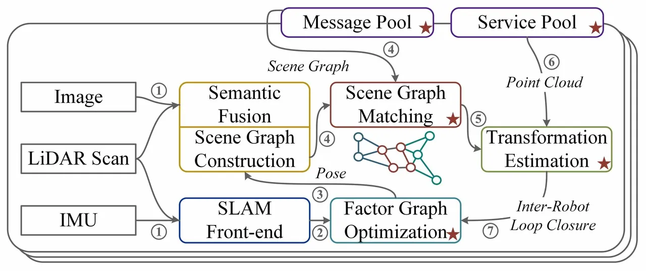
Figure 1: The paper's Fig. 3. Starred components cross the robot boundary; the remaining modules run locally on each platform.

The order matters: build semantic geometry locally, exchange only object summaries, and request heavy point clouds only after a match looks reliable. SGM-SLAM does not merely compress all messages. It uses the cheapest representation to decide whether an expensive registration is worth attempting.

flowchart TB
    A[LiDAR + IMU + RGB] --> B[Point-LIO odometry]
    A --> C[Oneformer image segmentation]
    B --> D[Keyframe layer]
    C --> E[Project points by intrinsics and extrinsics]
    E --> F[Semantic point layer]
    F --> G[Cluster bounded objects]
    D --> H[Object layer]
    G --> H
    H -->|IDs, labels, centroids| I[Neighbor object graph]
    H --> J[Local object graph]
    I --> K[Scene graph matching]
    J --> K
    K -->|enough matches| L[Coarse rigid transformation]
    L --> M[ICP on sparse matched object clouds]
    M --> N[Inter-robot factors]
    B --> O[Local pose graph optimization]
    D --> O
    N --> O
    O -->|pose updates| H
  

Figure 2: Data flow in SGM-SLAM. Lightweight object messages pass through the matching gate before keyframes and compressed point clouds are requested.

Scene Graph Construction

The scene graph has three layers. The keyframe layer contains keyframes selected by the SLAM front end; its edges include odometry, intra-robot loops, and inter-robot observations. The object layer is a fully connected undirected graph whose vertices are objects and whose edge weights are Euclidean distances between centroids. The semantic layer stores labeled point clouds and connects each scan to the keyframe during which it was captured. Cross-layer links relate a keyframe to every object observed there.

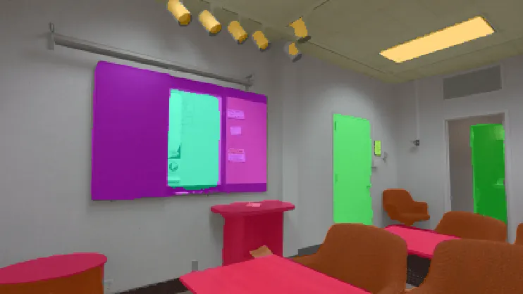
Figure 3: The paper's Fig. 4. Oneformer segments the RGB image, LiDAR points are projected into the image, and detected objects connect to the keyframe layer.

Object construction begins with Oneformer segmentation on RGB images. The authors intentionally segment only image data to keep semantic labels consistent; they do not run a separate 3D semantic predictor. LiDAR points are projected into the RGB frame using LiDAR-camera extrinsics and camera intrinsics. Each point receives the label of the nearest pixel. The labeled points are then clustered into bounded objects. This division of labor lets the 2D segmentation model supply semantic identity while LiDAR supplies geometric extent.

Maintaining the same object across keyframes is formulated as a linear assignment problem. Let $\mathcal{V}_\alpha^{(t)}$ and $\mathcal{V}_\alpha^{(t-1)}$ be object candidates at the current and previous keyframes. With assignment matrix $A_n$, cost matrix $C$, and centroid distance $c_{ij}=\lVert p_i-p_j\rVert_2$, the system solves

$$A_n^{*}=\arg\min_{A_n}\sum C\odot A_n,$$

$$A_n^{*}=\arg\min_{A_n}\sum_{v_i\in\mathcal{V}_\alpha^{(t)}}\sum_{v_j\in\mathcal{V}_\alpha^{(t-1)}}c_{ij}\cdot a_{ij},$$

$$\text{s.t.}\quad \forall v_j\in\mathcal{V}_\alpha^{(t-1)},\sum_{v_i\in\mathcal{V}_\alpha^{(t)}}a_{ij}\leq 1,\quad \forall v_i\in\mathcal{V}_\alpha^{(t)},\sum_{v_j\in\mathcal{V}_\alpha^{(t-1)}}a_{ij}\leq 1.$$

$A_n$ is Boolean, and $a_{ij}=1$ means that current object $v_i$ and historical object $v_j$ are associated. The inequalities permit an unmatched row or column, so new objects can enter and disappeared objects need not be forced into an incorrect association. A match is accepted only when $a_{ij}=1$ and $c_{ij}<c_{\max}$, where $c_{\max}$ bounds plausible object motion between keyframes. The Hungarian algorithm solves the assignment.

This layer is more than object bookkeeping. If local tracking fragments one physical chair into several vertices, the later edge-length signature loses its global geometry. The hierarchy also provides a propagation path: after a pose-graph correction changes keyframe poses, each object is updated according to the latest keyframe that observes it. The object layer therefore remains synchronized with optimized state estimates rather than becoming a stale detection log.

Inter-Robot Scene Graph Matching

Direct centroid comparison is impossible because $\mathcal{G}_\alpha$ and $\mathcal{G}_\beta$ are expressed in different world frames. SGM-SLAM represents a selected object as $\phi(v_i)=(p_i,l_i)$, where $p_i$ is its centroid and $l_i$ its semantic class. Edge $e_{ij}$ has weight $w_{ij}=\lVert p_i-p_j\rVert_2$. Only selected classes participate: the authors note that centroids of large objects can shift substantially when only part of the object is observed from different viewpoints.

The inter-robot problem is a quadratic assignment problem. For local graph $\mathcal{G}_\alpha=\langle\mathcal{V}_\alpha,\mathcal{E}_\alpha\rangle$ and neighbor graph $\mathcal{G}_\beta=\langle\mathcal{V}_\beta,\mathcal{E}_\beta\rangle$, assignment matrix $A_e$ scores pairs of edges rather than isolated vertices:

$$A_e^{*}=\arg\max_{A_e}\sum A_e\odot U\odot A_e,$$

$$A_e^{*}=\arg\max_{A_e}\sum_{v_i,v_j\in\mathcal{V}_\alpha}\sum_{v_m,v_n\in\mathcal{V}_\beta}a_{im}\cdot u_{ijmn}\cdot a_{jn},$$

$$\text{s.t.}\quad \forall v_i\in\mathcal{V}_\alpha,\sum_{v_m\in\mathcal{V}_\beta}a_{im}\leq 1,\quad \forall v_m\in\mathcal{V}_\beta,\sum_{v_i\in\mathcal{V}_\alpha}a_{im}\leq 1.$$

The entry $a_{im}\in\{0,1\}$ indicates whether local vertex $v_i$ matches neighbor vertex $v_m$. The four-dimensional utility tensor is

$$u_{ijmn}=d_v(v_i,v_m)\cdot d_v(v_j,v_n)\cdot d_e(e_{ij},e_{mn}),$$

$$d_e(e_{ij},e_{mn})=\exp(-\mu\lvert w_{ij}-w_{mn}\rvert).$$

In this implementation, $d_v$ compares only semantic labels: it is 1 when the labels agree and 0 otherwise. The edge term penalizes differences between inter-object distances, with $\mu$ controlling geometric strictness. A single incorrect endpoint zeroes the product. A pair of edges whose lengths differ greatly receives exponentially less support. This is the precise meaning of the paper's claim that matching uses only object labels and centroids: no visual descriptor, color histogram, or learned appearance embedding is transmitted.

To make the combinatorial problem tractable, the authors vectorize $A_e$ into $\text{vec}(A_e)$ and reshape $U$ into $U_{\text{2D}}$:

$$A_e^{*}=\arg\max_{A_e}\text{vec}(A_e)^\top\cdot U_{\text{2D}}\cdot\text{vec}(A_e).$$

The Boolean constraint is relaxed to $a_{ij}\in[0,1]$. Following the spectral matching argument of Leordeanu et al., $A_e^{*}$ is taken as the positive eigenvector of $U_{\text{2D}}$ associated with its principal eigenvalue. The system then performs one more linear assignment with cost $C=-A_e^{*}$ to recover discrete object matches, using a minimum eigenvector value to reject weak evidence. The relaxation gives up exact 0/1 combinatorial optimality but yields a practical approximation for online robots.

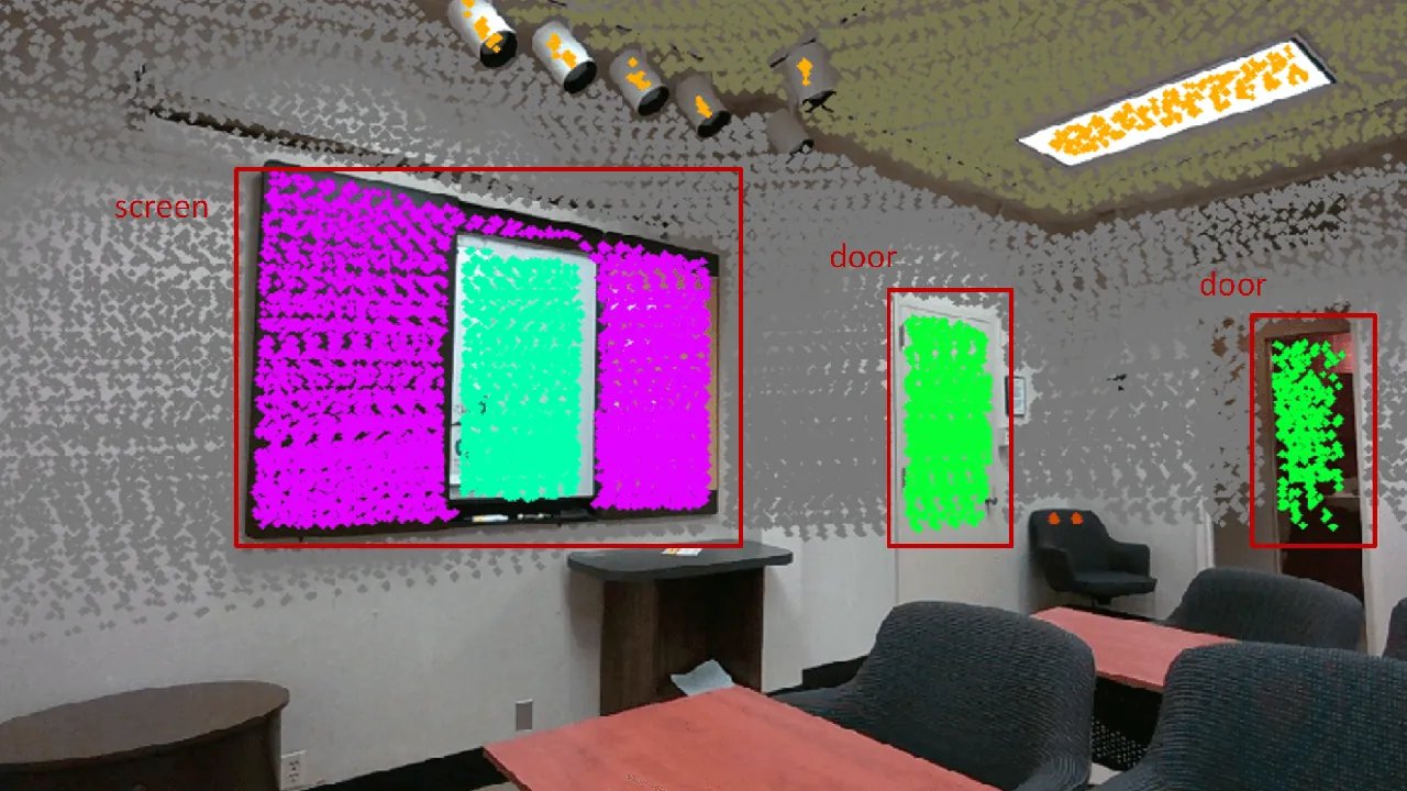
Figure 4: The paper's Fig. 5. Node colors encode classes and edge lengths encode weights; only label-compatible, length-compatible edges receive high utility.

The representation has a clear physical rationale. Image descriptors depend on projected appearance. Distances among rigid objects survive a rigid coordinate transform. A semantic label only needs the segmentation model to agree across views; it does not need identical texture, illumination, or image scale. That makes the method suitable for different sensor heights, occlusion by vegetation, low-overlap trajectories, and changing light. The cost is ambiguity in repetitive scenes. When many same-class objects have similar pairwise distances, label and edge length alone may admit multiple explanations, so the system must rely on a minimum number of matches and later point-cloud refinement.

From Object Matches to a Transform

Let $\mathcal{A}_{\alpha,\beta}$ denote matched vertex pairs. For every pair, centroids $p_\alpha$ and $p_\beta$ satisfy

$$\begin{bmatrix}p_\alpha\\1\end{bmatrix}=\mathbf{T}_{\mathbf{W}_\alpha\rightarrow\mathbf{W}_\beta}\begin{bmatrix}p_\beta\\1\end{bmatrix}.$$

More than three non-collinear objects are sufficient to estimate a rigid transform. The authors add a practical prior: objects are assumed to lie approximately on a plane. This reduces the solve to a 2D rigid transform and avoids tilting caused by odometric drift or inconsistent vertical centroid estimates. The assumption fits tables, benches, and chairs placed near the ground, which are common in both experiments.

This transform is only an initial guess. Centroids depend on segmentation boundaries, occlusion extent, and viewpoint. A planar solve also discards height information in stairways, ramps, and vertically extended structures. SGM-SLAM therefore uses it to initialize inter-robot point-cloud registration. In the scene graph, each object vertex $v$ references keyframes $\mathcal{F}_v=\{F(i)\}$ where it was observed. The local target cloud is

$$M_{v_\alpha}=\bigcup_i F_{v_\alpha}(i).$$

For neighbor object $v_\beta$, the source uses a sliding window around each relevant keyframe $F_{v_\beta}(j)$:

$$M_{v_\beta}=\bigcup_{k=-5}^{5}F_{v_\beta}(j+k).$$

The source cloud is transformed by $\mathbf{T}_{\mathbf{W}_\alpha\rightarrow\mathbf{W}_\beta}$ and registered to the target with ICP. The resulting constraints enter the local factor graph. To keep computation bounded, each neighbor keyframe is registered with only one local keyframe. The architecture therefore avoids a brute-force all-pairs point-cloud search: graph matching supplies correspondence, centroids supply initialization, and sparse object geometry supplies refinement.

Communication Protocol

Communication occurs in three stages. First, robots continuously share the lightest data: object ID, type, and centroid. These updates are sent only after a significant scene-graph change, such as a new object or a large drift correction, so their rate is much lower than the LiDAR rate. Second, when a robot finds enough matched objects, it requests the sparse object point clouds and associated keyframe IDs for those matches. Third, it requests any required keyframes it has not stored, receiving compressed point clouds, optimized state estimates, and marginalized covariances.

Transmitted point clouds keep geometry only; intensity and color are omitted. They are compressed with the Point Cloud Library. The requester confirms which keyframes it has already received to avoid duplicates. The authors still observed a burst problem in real data: once scene graphs matched, many similar keyframe requests were generated, old requests were dropped, and requests outnumbered responses. They propose a delayed request strategy as future work. This is an important protocol lesson. Average bandwidth savings do not automatically eliminate bursts triggered by a successful match.

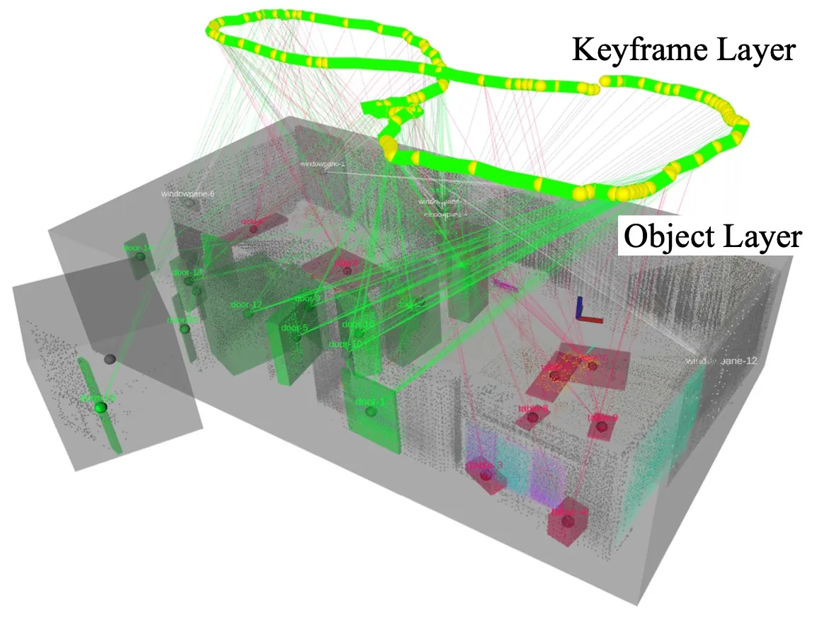
Figure 5: The paper's Fig. 6. The Unitree quadruped carries the same sensing package as the handheld rig: Livox mid-360, IMU, and RealSense RGB camera.

Synthetic Matching Evaluation

The synthetic experiment isolates graph matching and transform estimation. A $60\text{ m}\times60\text{ m}$ environment contains 50 objects from 6 classes, with random poses and dimensions. Each condition is repeated 20 times with random initial transforms. Estimation is successful when translation error $e_t<2\text{ m}$ and per-axis rotation error $e_r<20^\circ$. In the perturbed setting, centroid positions receive uniform errors of $\pm1\text{ m}$ along $x$ and $y$ and $\pm0.5\text{ m}$ along $z$; orientation receives $\pm2.5^\circ$ roll and pitch and $\pm10^\circ$ yaw.

The first table varies graph size and overlap. With 8, 15, and 35 objects in the first graph and 4, 7, and 17 overlapping objects, success is 100% without centroid error. Under centroid and orientation perturbation, only the 4-object-overlap case degrades, to 65%. Recall remains 100% in all three rows. Runtime grows from 7 ms to 226 ms as the graphs enlarge, but remains compatible with an online matching step.

Graph 1 objects	Graph 2 objects	Overlap	Success, no error	Success, with error	Recall, no/with error	Runtime
8	8	4	100%	65%	100% / 100%	7 ms
15	15	7	100%	100%	100% / 100%	14 ms
35	32	17	100%	100%	100% / 100%	226 ms

Table 1: Synthetic results from the paper's Table 1, without semantic label errors.

The second table isolates semantic noise. Both graphs contain 35 and 32 objects, with 17 overlapping. With 3 or 6 mislabeled objects, success remains 100%. At 9 mislabels it falls to 95%. At 12, success is only 55% without pose error and 30% when pose error is added. Aggregate recall falls from 82% to 27%. The pattern is informative: edge-length structure absorbs a small number of wrong labels, but incorrect labels remove high-utility edges. Once a large fraction of overlapping evidence is corrupted, the spectral matching gate becomes unreliable.

Mislabeled objects	Success, no pose error	Success, with pose error	Recall, no/with pose error	Runtime
3	100%	100%	82% / 82%	209 ms
6	100%	100%	63% / 59%	188 ms
9	95%	95%	46% / 46%	183 ms
12	55%	30%	29% / 27%	178 ms

Table 2: Semantic mislabeling stress test from the paper's Table 2.

The paper's Fig. 7 illustrates why the method is not a strict node classifier. A table misclassified as a sofa does not prevent a successful transform because other object pairs still support a consistent edge-length configuration. Matching searches for the highest-scoring global structure. Yet the synthetic setup also has a boundary: it assumes object graphs already exist and does not simulate missed detections, object merges, moving people, or time synchronization faults. Its numbers should be read as stress on the matcher, not as end-to-end field success.

Real-World SLAM Results

The real platform pairs a handheld device and a Unitree Go2 EDU quadruped. Both carry Livox mid-360 LiDAR, an inertial sensor, and an Intel RealSense depth camera, but only the RGB stream is used. The quadruped's onboard sensors are not part of the pipeline; the same handheld package is mounted on top. The authors collected a new dataset because prior multi-robot sets often use Velodyne VLP-16 scans, whose sparse layered structure does not directly suit the clustering-based object detector used with denser Livox data. The system runs ROS 2 Foxy on Ubuntu 20.04, and GPU use is limited to image segmentation.

The outdoor sequence has two robots over a larger campus area, sparse man-made objects, trees, and little trajectory overlap. The indoor sequence has three robots over a smaller area, dim lighting, and many repeated chairs, tables, and bookshelves. Neither sequence has GPS because of equipment limitations. The authors use COLMAP structure-from-motion as ground truth, reconstructing only feature-rich regions so that inter-robot relative poses are reliable. The distributed comparison baseline is Swarm-SLAM with RTAB-Map LiDAR odometry. Swarm-SC uses Scan Context; Swarm-CP uses CosPlace.

Environment	Swarm-SC ATE RMSE	Swarm-CP ATE RMSE	SGM-SLAM ATE RMSE
Outdoor	20.29 m	3.92 m	1.32 m
Indoor	3.36 m	5.70 m	0.81 m

Table 3: Absolute trajectory error from the paper's Table 3. Multiple robot trajectories are combined for EVO evaluation.

The mechanism behind the numbers matters more than the ranking. Outdoor Swarm-SC fails where scans overlap too little for Scan Context to form a reliable signature. Indoor Swarm-CP fails where lighting and sensor-height differences weaken image retrieval. SGM-SLAM reaches 1.32 m outdoors and 0.81 m indoors by using a representation that changes the evidence being compared: sparse but stable object identity and object-to-object geometry. The same object graph can bridge little overlap outdoors and repetitive structure indoors.

The ground truth should temper the interpretation. COLMAP globally optimizes image observations, but the authors reconstruct only feature-rich areas, so ATE is measured only there. SfM is not infallible in weak texture or dynamic scenes. Even so, all three methods are evaluated against the same reference, and the selected scenes deliberately contain the failure conditions that the object graph is intended to address. The result is therefore targeted evidence rather than a universal benchmark.

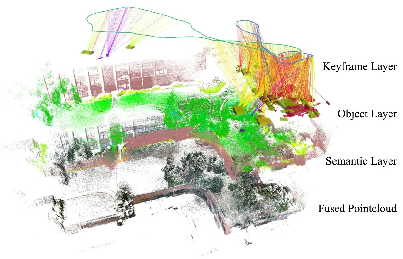
Figure 6: The paper's Fig. 1. Blue and green trajectories form the keyframe layer, colored boxes form the object layer, and semantically segmented points form the semantic layer.

Communication Analysis

The communication experiment uses simulated wireless communication over the real datasets. The raw point-cloud baseline represents a brute-force centralized policy in which every scan is sent to a server. Outdoor raw messages average 508.2 KB and occur 3073 times; indoor raw messages average 508.1 KB and occur 3079 times. Object data is much smaller and less frequent: 7.76 KB mean over 701 messages outdoors, and 18.40 KB mean over 845 indoors. Object data alone totals roughly 5.4 MB outdoors and 15.5 MB indoors, while both raw baselines are near 1.56 GB.

Message type	Environment	Mean	Maximum	Count
Raw point cloud	Outdoor	508.2 KB	516.9 KB	3073
Raw point cloud	Indoor	508.1 KB	512.1 KB	3079
Object data	Outdoor	7.76 KB	16.93 KB	701
Object data	Indoor	18.40 KB	44.37 KB	845
Keyframe request	Outdoor	0.02 KB	0.02 KB	61
Keyframe request	Indoor	0.02 KB	0.02 KB	411
Keyframe response	Outdoor	18.87 KB	22.95 KB	10
Keyframe response	Indoor	6.90 KB	11.05 KB	72

Table 4: Perception message statistics from the paper's Table 4. Compressed point clouds contain geometry but no color or intensity.

The request/response imbalance deserves as much attention as the byte totals. Outdoor runs contain 61 requests but only 10 responses; indoor runs contain 411 requests but 72 responses. The authors attribute this to repeated burst requests after scene graphs match, causing older requests to be dropped. A practical deployment therefore needs request deduplication, pacing, priority, or delayed confirmation. Without that scheduling layer, the benefit of on-demand point clouds can be consumed exactly when matching succeeds.

Limitations

The first author-stated limitation is data collection. Because equipment was unavailable, each sequence was recorded separately as a ROS 2 bag and synchronized offline by simultaneous playback; GPS was unavailable in both environments. Ground truth comes from COLMAP SfM over feature-rich areas. This supports relative-pose evaluation but does not exercise online wireless latency, packet loss, or simultaneous multi-robot clock uncertainty.

The second author-stated limitation is request scheduling. Keyframe requests greatly outnumber responses because a successful match triggers many similar requests and old requests are dropped. The authors explicitly propose delayed request optimization. This is not a failure of matching accuracy; it is a protocol-layer failure mode that emerges when lightweight matching succeeds and immediately creates demand for heavy data.

A method boundary follows from the matching evidence itself. Only labels and edge lengths are compared, mainly because large-object centroids can vary under partial observation. This choice helps with viewpoint changes but can become ambiguous in repeated environments. Table 2 quantifies the sensitivity: 12 mislabels reduce success to 55% without pose error and 30% with pose error. Real deployments add missed detections, moving pedestrians, segmentation instability, and seasonal appearance changes that are not separately ablated.

The planar rigid-transform prior is another boundary. It suppresses roll and pitch errors from odometry and works for ground-level furniture, but it discards height information in ramps, stairs, slopes, and vertically extended objects. Sparse ICP can correct some initial error, yet a degraded planar initialization may still lead registration into a local minimum.

Finally, the distributed choice not to share detected inter-robot observations reduces synchronization but leaves local estimates potentially inconsistent. Each robot optimizes only the neighbor states it has associated. The paper does not analyze covariance consistency, repeated encounters, or arbitration when two robots infer conflicting relative transforms.

Engineering Takeaways

For multi-robot system designers, SGM-SLAM is valuable as a pattern as much as a result: summarize the scene cheaply, use that summary to decide where heavy alignment is plausible, and fetch only the geometry needed to confirm it. The same ordering can guide heterogeneous inspection fleets, search-and-rescue teams, and deployments over intermittent 4G/5G or constrained robot-to-radio links.

The work also shows that a scene graph need not be only a human-facing output. When nodes retain geometric relations, the graph participates in localization. A later LLM or task planner can query rooms, chairs, benches, and work areas without a separate semantic index. The conclusion names LLM-based motion planning as future work, but the evaluated system remains focused on state estimation and map merging, not open-vocabulary perception or language-conditioned tasks.

Reproduction requires several specific choices. Oneformer performs image segmentation; Point-LIO supplies odometry; intra-robot loops use a LIO-SAM-like distance rule; PCL compresses geometry-only point clouds. The implementation uses ROS 2 Foxy on Ubuntu 20.04. Because no public code or pending repository is listed, an engineering reimplementation must also design the object lifecycle, communication state machine, and request deduplication.

Conclusion

SGM-SLAM compresses inter-robot association to semantic labels and centroid-derived graph structure, then uses a staged pipeline of graph matching, coarse rigid estimation, and sparse ICP. The synthetic study quantifies how much overlap and semantic noise the matcher tolerates. Real experiments report 1.32 m outdoor and 0.81 m indoor ATE RMSE, outperforming the evaluated Swarm-SLAM descriptor configurations. Communication tables reduce raw-point-cloud traffic near 1.56 GB to several to tens of megabytes of object data, while also exposing the burst-request problem that remains unsolved.

The boundaries are equally clear. The method assumes stable object classes, mostly planar object layouts, and a wireless link that can absorb post-match bursts. The most useful next work is not necessarily another larger descriptor, but open-vocabulary object stability, height-aware transform estimation, distributed consistency across repeated encounters, and realistic request scheduling under lossy links.