UniSim-SLAM: Feed-Forward SLAM with Unified Sim(3) Optimization

Paper Metadata

Item	Detail
Title	UniSim-SLAM: Feed-Forward SLAM with Unified Sim(3) Optimization
Authors	Inha Lee, Dongjae Jeong, Junhee Lee, Kyungdon Joo (corresponding author) - UNIST, Ulsan, South Korea
arXiv	2608.01706v1 (2026-08-03, cs.CV), accepted to ECCV 2026
Code	Not released yet. The official repository vision3d-lab/UniSim-SLAM exists but contains only a README reading "comming soon" (no implementation as of 2026-09); the project page vision3d-lab.github.io/unisim-slam likewise states "Code Coming soon", so this entry records a pending status
Benchmarks	TUM RGB-D, 7-Scenes (with the revised ground-truth poses of Brachmann et al.), Replica
Frontend backbone	VGGT (default, one shared model for both two-view and multi-view inference); swappable for the low-latency STA

One-Sentence Summary

Port the classic SLAM split of a lightweight odometry frontend and an optimizing backend onto feed-forward geometric foundation models: two-view inference handles low-latency frame-by-frame tracking, multi-view submaps supply rich corrective constraints, and the heterogeneous, scale-inconsistent local frames produced by both are optimized jointly inside a single $Sim(3)$ multi-level factor graph. Under the uncalibrated protocol this drives TUM RGB-D trajectory error down to 0.032 m (38.5% below the previous best) and 7-Scenes to 0.020 m (45.9% below).

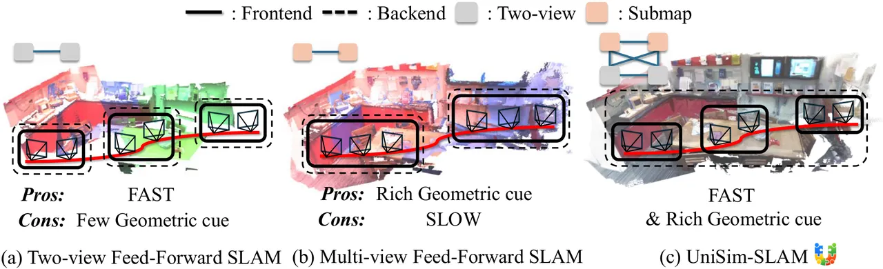
Figure 1: The paper teaser. (a) Two-view inference is cheap but geometrically under-constrained; (b) multi-view submap inference is geometry-rich yet must accumulate frames first, so latency is high; (c) UniSim-SLAM combines a two-view frontend with a multi-view submap backend and optimizes both in one unified $Sim(3)$ factor graph.

Background and Motivation

Geometric foundation models such as DUSt3R and VGGT made feed-forward SLAM possible for the first time: given a few uncalibrated images, a single network pass returns dense depth maps and relative poses, with no hand-designed feature matching and no per-sequence re-optimization. A wave of systems built on that capability, wiring it into a SLAM pipeline. MASt3R-SLAM runs real-time dense monocular SLAM with a two-view model, ViSTA-SLAM pairs a symmetric two-view associative frontend with a $Sim(3)$ pose-graph backend, and VGGT-SLAM incrementally builds VGGT submaps while optimizing a 15-DoF projective transform on the $SL(4)$ manifold to absorb the ambiguities introduced by missing calibration.

The authors point out a structural nuisance that these systems largely gloss over: the geometric estimate of a feed-forward model is conditioned on the input view configuration. Feed the same image together with different co-visible frames and the recovered scale and pose both change. Stringing successive feed-forward outputs together over a long sequence therefore concatenates a set of local reconstructions, each defined in its own frame and each carrying its own scale, which is exactly where geometric inconsistency and trajectory drift come from. A global trajectory can only be recovered by aligning those configuration-dependent local reconstructions one by one. Two-view methods align pairwise reconstructions through mutual constraints; multi-view methods register submaps by estimating transforms in overlapping regions.

Beyond that configuration-dependent inconsistency, relying on a single inference paradigm runs into a fundamental trade-off (Figure 1). Multi-view inference is rich in constraints but needs a fixed number of frames (one submap) before it can run at all, so per-frame updates are out of reach; and refining purely through inter-submap relations requires neighbouring submaps to overlap so that corrections can propagate along the trajectory, otherwise geometric fixes never leave their neighbourhood. Two-view inference is the mirror image: light, available as soon as one frame arrives, naturally temporally connected, but so weakly constrained that drift accumulates and long-horizon global consistency cannot be sustained.

The authors break the deadlock by looking back at classical SLAM. ORB-SLAM, LSD-SLAM, Kimera and DSO resolved the same efficiency-versus-consistency trade-off long ago with a cheap two-view odometry frontend plus an intermittently invoked globally consistent backend. The temporal coherence of the two-view frontend keeps the graph connected, while the multi-view submaps of the backend provide rich geometric constraints. The trouble is that existing feed-forward methods do either pairwise two-view alignment or inter-submap registration, never both; and naively gluing the two kinds of prediction together is not trivial, because they live in heterogeneous local frames with mismatched scales and reference frames. A new factor-graph formulation is required to optimize them within one framework.

That yields the core insight of the paper: geometric predictions produced by different feed-forward inference paradigms can be read as complementary constraints residing in heterogeneous local frames, and therefore have to be optimized jointly in a single unified $Sim(3)$ factor graph. Two-view inference contributes lightweight, densely connected temporal constraints that sustain low-latency tracking, while multi-view inference yields geometrically coherent submaps that anchor the global scene structure. The $Sim(3)$ manifold, which admits rotation, translation and scale ambiguity at once, is precisely the right stage for hosting both kinds of constraint.

Preliminaries: Sim(3) and Feed-Forward Geometric Models

$Sim(3)$ is the group of 3D similarity transforms. One element encodes a scale $s\in\mathbb{R}^{+}$, a rotation $R\in SO(3)$ and a translation $t\in\mathbb{R}^{3}$ simultaneously, represented as a $4\times4$ homogeneous matrix. Compared with the rigid $SE(3)$, the extra scale dimension is exactly what an uncalibrated monocular setting demands: the absolute scale of a monocular reconstruction is unobservable, and the depth returned by a feed-forward model is only determined up to a scale factor. Every pose variable and residual in this paper is defined on $Sim(3)$ and its Lie algebra $\mathfrak{sim}(3)$, and residuals are pulled into the algebra with the logarithmic map $\log(\cdot)$ before least-squares optimization.

The system uses two kinds of feed-forward inference. Two-view inference $f_{\text{2v}}$ takes an adjacent keyframe pair and returns two depth maps plus a relative transform; multi-view inference $f_{\mathrm{mv}}$ takes a window of consecutive keyframes and returns the submap-local depth and pose of every frame inside it. Both call the same geometric foundation model (VGGT by default) and differ only in how many views they ingest and which thread they run on. The authors deliberately use the distinct notation $f_{\text{2v}}$/$f_{\mathrm{mv}}$ to underline that the backend executes asynchronously.

Method

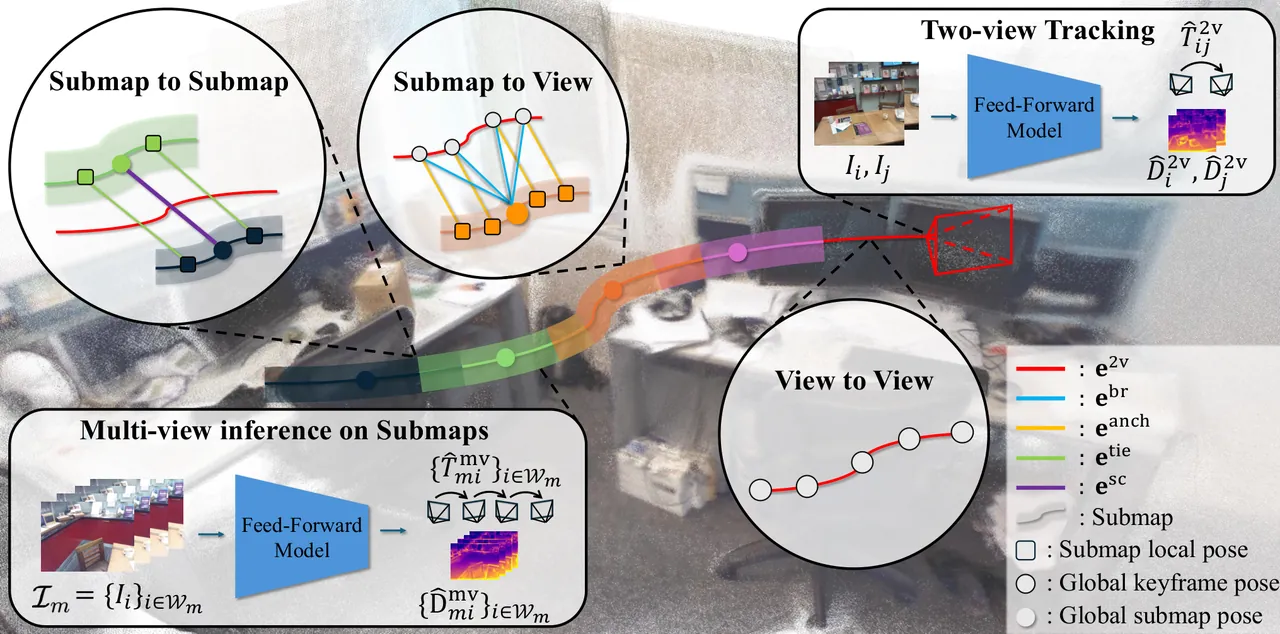
Figure 2: The overall framework. One feed-forward model produces both the two-view poses/depths used for tracking and the multi-view submap predictions used for local geometry; these predictions are integrated into a unified $Sim(3)$ factor graph with several edge types, which jointly optimizes global keyframe poses and submap poses.

1. Frontend: Two-View Tracking on Keyframes

The frontend is responsible for low latency and temporal coherence. For every temporally adjacent keyframe pair $(I_{i},I_{j})$ (with $j=i+1$), the image pair goes into the feed-forward model to obtain the two-view estimate:

$$\{\hat{D}^{\text{2v}}_{i},\hat{D}^{\text{2v}}_{j},\hat{T}^{\text{2v}}_{ij}\}=f_{\text{2v}}(I_{i},I_{j})$$

Here $\hat{D}^{\text{2v}}$ is the predicted depth map and $\hat{T}^{\mathrm{2v}}_{ij}\in Sim(3)$ is the relative transform from $I_i$ to $I_j$, whose scale component is initialized to 1. Those depth maps come back later: they are the raw material for estimating scale anchors during submap integration.

To assemble a global trajectory from these relative measurements the authors first fix a global reference frame, taking the very first keyframe $I_0$ as the origin of the global coordinate system. They then compose the two-view relative transforms sequentially and online to initialize the global poses:

$$T_{j}=T_{i}\hat{T}^{\mathrm{2v}}_{ij}$$

This step looks naive but implicitly defines the temporal edges of the pose graph and keeps it connected, even when submaps do not overlap at all. The resulting trajectory is only an initial guess, later refined by the multi-view submap constraints of the backend.

2. Backend: Multi-View Submap Integration

The backend must correct the drift accumulated in the global keyframe poses $\{T_i\}$. Once enough consecutive keyframes have piled up, one multi-view inference is run on the consecutive window $\mathcal{W}_{m}\subset\{1,\dots,N\}$ belonging to the $m$-th submap:

$$\{\hat{D}^{\mathrm{mv}}_{mi},\hat{T}^{\mathrm{mv}}_{mi}\}_{i\in\mathcal{W}_{m}}=f_{\mathrm{mv}}(\mathcal{I}_{m})$$

$\hat{T}^{\mathrm{mv}}_{mi}\in Sim(3)$ is the pose of $I_i$ inside the local frame of submap $m$ (again with unit initial scale), and the submap origin is placed at the central frame of the window. To attach this local reconstruction to the global trajectory the authors introduce a submap pose $S_{m}\in Sim(3)$ mapping the frame of submap $m$ into the global frame, which gives the consistency relation:

$$T_{i}\approx S_{m}\hat{T}^{\text{mv}}_{mi}$$

There is an easy-to-skip point here: because a multi-view prediction depends on the view set, the same keyframe shows up in different submaps with different scale and pose. Submap-local poses can therefore never be consumed directly as globally consistent measurements, and the extra layer of variables $\{S_m\}$ is mandatory.

Before joint optimization $S_m$ needs an initial value. Let $I_i$ be the origin keyframe of submap $m$ (so $\hat{T}^{\mathrm{mv}}_{mi}=\mathbf{I}$), whose global pose from two-view inference is

$$T_{i}=\begin{bmatrix}s_{i}R_{i}&t_{i}\\ \mathbf{0}^{\top}&1\end{bmatrix}$$

To dissolve the relative-scale ambiguity between the two-view and multi-view predictions the authors estimate a relative scale from depth statistics, $s^{\mathrm{rel}}_{mi}=\mathrm{median}(\hat{D}^{\mathrm{mv}}_{mi}/\hat{D}^{\mathrm{2v}}_{i})$: a per-pixel ratio followed by a median, which is naturally robust to local depth errors. Since the multi-view prediction is expressed at unit scale, the initial submap scale is $s_{m}^{(0)}=s_{i}/s^{\mathrm{rel}}_{mi}$, hence

$$S_{m}^{(0)}=\begin{bmatrix}s_{m}^{(0)}R_{i}&\dfrac{t_{i}}{s^{\mathrm{rel}}_{mi}}\\ \mathbf{0}^{\top}&1\end{bmatrix}$$

The translation is scaled by the same relative factor to keep the similarity-transform structure between the global and submap frames intact. This initialization embeds the submap consistently, at the right scale, into the global trajectory, after which $\{T_i\}$ and $\{S_m\}$ enter joint optimization together.

A single relative-scale constraint applied only at initialization is not enough, though: once two-view and multi-view constraints are active simultaneously, several $Sim(3)$ relations coexist inside one submap, with every keyframe carrying a global pose $T_i$ while the submap itself carries $S_m$. That is precisely what motivates the multi-level factor-graph formulation.

3. The Unified Sim(3) Pose Graph: Three Edge Types, Five Residuals

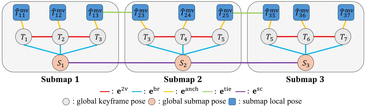
Figure 3: The structure of the multi-level factor graph (paper Fig. 3). Nodes come in two layers, global keyframe poses $\{T_i\}$ and submap poses $\{S_m\}$; edges come in three types, temporal, view-to-submap and submap-to-submap.

The node set of the unified graph $\mathcal{G}=(\mathcal{V},\mathcal{E})$ consists of global pose nodes and submap pose nodes:

$$\mathcal{V}=\mathcal{V}_{T}\cup\mathcal{V}_{S},\quad\mathcal{V}_{T}=\{T_{i}\in Sim(3)\},\quad\mathcal{V}_{S}=\{S_{m}\in Sim(3)\}$$

The edge set decomposes into three levels:

$$\mathcal{E}=\mathcal{E}^{\mathrm{temp}}\;\cup\;\mathcal{E}^{\mathrm{v2s}}\;\cup\;\mathcal{E}^{\mathrm{s2s}}$$

View-to-view (temporal) edges. $\mathcal{E}^{\mathrm{temp}}=\{(i,j)\mid j=i+1\}$; each edge corresponds to a pair of temporally adjacent keyframes and imposes $T_{i}^{-1}T_{j}\approx\hat{T}^{\mathrm{2v}}_{ij}$. Its residual in the Lie algebra $\mathfrak{sim}(3)$ is

$$\mathbf{e}^{\mathrm{2v}}_{ij}=\log\left((\hat{T}^{\mathrm{2v}}_{ij})^{-1}(T_{i}^{-1}T_{j})\right)$$

Their role goes beyond local consistency: these edges form the globally connected temporal backbone, and when submaps are sparse or mutually non-overlapping they are the only channel through which corrections from higher-level constraints propagate along the whole trajectory.

View-to-submap edges. $\mathcal{E}^{\mathrm{v2s}}=\{(m,i)\mid i\in\mathcal{W}_{m}\}$ connects a global pose node $T_i$ to the submap pose node $S_m$ it belongs to. Each edge carries two complementary residuals. The first is the pose-alignment (bridge) residual:

$$\mathbf{e}^{\mathrm{br}}_{mi}=\log\left((\hat{T}^{\mathrm{mv}}_{mi})^{-1}S_{m}^{-1}T_{i}\right)$$

Bridge edges align submap-local predictions with the global trajectory and remove drift inside the window $\mathcal{W}_m$; when a keyframe is shared by several submaps this coupling also aligns overlapping submaps implicitly through the shared global pose node. Pose alignment alone, however, does not constrain the relative scale between the global trajectory and the submap frame, which motivates the second residual, a scale anchor built from per-view depth statistics:

$$\mathbf{e}^{\mathrm{anch}}_{mi}=\log s_{i}-\log s_{m}-\log\left(\mathrm{median}(\hat{D}^{\mathrm{mv}}_{mi}/\hat{D}^{\mathrm{2v}}_{i})\right)$$

It operates in log-scale space and pins the relative scale to the median of the depth ratio, preventing scale inconsistency from spreading across submaps.

Submap-to-submap edges. Although view-to-submap edges let submaps align indirectly through global view nodes, that coupling can be compensated by moving the intermediate view node, so a degenerate solution exists. To enforce strict consistency between submap frames the authors connect overlapping-window submaps directly: $\mathcal{E}^{\mathrm{s2s}}=\{(m,n)\mid\mathcal{W}_{m}\cap\mathcal{W}_{n}\neq\emptyset\}$, with the shared keyframe set denoted $\mathcal{V}_{mn}=\mathcal{W}_{m}\cap\mathcal{W}_{n}$. For each shared frame $i$ the two submaps give independent local pose predictions, and geometric consistency requires that transforming from either submap frame yields the same global pose, i.e. the tie residual:

$$\mathbf{e}^{\mathrm{tie}}_{mni}=\log\left((S_{m}\hat{T}^{\mathrm{mv}}_{mi})^{-1}(S_{n}\hat{T}^{\mathrm{mv}}_{ni})\right)$$

A second residual enforces inter-submap scale consistency. Per-view relative scales $\hat{s}_{mn,i}=\mathrm{median}(\hat{D}^{\mathrm{mv}}_{mi}/\hat{D}^{\mathrm{mv}}_{ni})$ are first estimated for every shared frame and then aggregated over the shared views, $\hat{s}_{mn}=\mathrm{median}_{i\in\mathcal{V}_{mn}}\hat{s}_{mn,i}$, giving

$$\mathbf{e}^{\mathrm{sc}}_{mn}=\log s_{n}-\log s_{m}-\log\hat{s}_{mn}$$

Estimating inter-submap relative scale from statistics of pixel-aligned depth predictions is both robust and free of any extra feature matching. Tie and scale constraints together stop independently estimated submaps from drifting apart.

4. Objective and Solver

The five residual families are collected into one nonlinear least-squares problem, jointly optimizing $\{T_i\}$ and $\{S_m\}$ on the $Sim(3)$ manifold:

$$\underset{\{T_{i}\},\{S_{m}\}}{\arg\min}\;\sum_{(i,j)\in\mathcal{E}^{\mathrm{temp}}}\rho\left(\left\|\mathbf{e}^{2v}_{ij}\right\|\right)+\sum_{(m,i)\in\mathcal{E}^{\mathrm{v2s}}}\Big(\rho\left(\left\|\mathbf{e}^{\mathrm{br}}_{mi}\right\|\right)+\rho\left(\left\|\mathbf{e}^{\mathrm{anch}}_{mi}\right\|\right)\Big)+\sum_{(m,n)\in\mathcal{E}^{\mathrm{s2s}}}\Big(\sum_{i\in\mathcal{V}_{mn}}\rho\left(\left\|\mathbf{e}^{\mathrm{tie}}_{mni}\right\|\right)+\rho\left(\left\|\mathbf{e}^{\mathrm{sc}}_{mn}\right\|\right)\Big)$$

$\rho(\cdot)$ is a Huber loss that suppresses the occasional outlier prediction of the feed-forward model; the solver is Levenberg-Marquardt running on the Lie algebra $\mathfrak{sim}(3)$. All experiments use one fixed set of residual weights:

$$(w^{\text{2v}},w^{\text{br}},w^{\text{anch}},w^{\text{sc}},w^{\text{tie}})=(1.0,1.0,50.0,50.0,0.2)$$

This weight allocation says a lot about the authors' design priorities. The two scale-related constraints ($w^{\text{anch}}$, $w^{\text{sc}}$) get a 50x boost because scale consistency is exactly where uncalibrated feed-forward SLAM tends to collapse; the tie constraint gets only 0.2, meaning the optimizer prefers to trust view-to-submap edges over direct submap-to-submap alignment when integrating local submap predictions. The weight ablation in Appendix A1 confirms this reading: lowering the scale weight from 50 to 1 degrades the 7-Scenes average ATE from 0.020 to 0.025, while raising the tie weight from 0.2 to 2.0 degrades it to 0.022.

flowchart TD
  IN["Image stream"] --> KF["Keyframe sampling
stride 5 (7-Scenes) / 3 (TUM)"]
  KF --> F2V["Frontend thread: f_2v
two-view depth + relative Sim(3)"]
  F2V --> COMP["Sequential composition
T_j = T_i * T_hat^2v_ij"]
  COMP --> INIT["Global keyframe poses T_i
(initial estimate)"]
  KF --> ACC{"14 new keyframes
accumulated?"}
  ACC -->|yes| FMV["Backend thread: f_mv
multi-view submap, w=16, phi=2"]
  FMV --> DSTAT["Depth-statistic relative scale
s_rel = median(D_mv / D_2v)"]
  DSTAT --> SMINIT["Submap pose init S_m^(0)"]
  INIT --> GRAPH["Unified Sim(3) factor graph"]
  SMINIT --> GRAPH
  GRAPH --> E1["E_temp: e_2v (w=1.0)"]
  GRAPH --> E2["E_v2s: e_br (w=1.0) + e_anch (w=50)"]
  GRAPH --> E3["E_s2s: e_tie (w=0.2) + e_sc (w=50)"]
  E1 --> LM["Huber + Levenberg-Marquardt
on sim(3)"]
  E2 --> LM
  E3 --> LM
  SALAD["SALAD retrieval
+ VGGT geometric verification"] --> LOOP["Joint loop submap"]
  LOOP --> GRAPH
  LM --> OUT["Refined T_i and S_m
global trajectory + dense map"]
  OUT -.->|"async, non-blocking"| F2V

5. Loop Closure

Long-term drift is caught by a loop-closure module that follows the VGGT-SLAM recipe but is plugged into the new graph. Loop candidates are retrieved with SALAD global image descriptors: for each query keyframe the most similar historical keyframe is taken, and it is accepted as a candidate only when the similarity exceeds a preset threshold. A geometric verification step then filters out matches that "look alike but make no geometric sense": the query and retrieved frames are handed to VGGT to estimate their relative geometry, and the candidate is rejected if the relative translation is implausibly large or the two-view field-of-view overlap is insufficient.

Once verification passes, the authors build a joint loop submap around the two matched keyframes: the two multi-view sets centred on the query frame and on the matched frame are aggregated and fed into one multi-view inference, and the resulting predictions are inserted as extra constraints into the unified $Sim(3)$ pose graph, pulling the whole trajectory back into consistency. Notably, loop closure is not a special branch in this framework; it is simply "produce one more submap node", and it runs through exactly the same edges and residuals.

6. Asynchronous Frontend and Backend

Frontend and backend run on separate threads and never block each other. The frontend performs two-view estimation for every incoming keyframe at roughly 25 FPS on 7-Scenes, while the backend fires only after enough new keyframes have accumulated (14 new keyframes in the default configuration). This asynchronous design brings one practical degree of freedom: $f^{\text{2v}}$ and $f^{\mathrm{mv}}$ need not be the same model, because the global trajectory is refined by $Sim(3)$ optimization over depth and pose, so the frontend can be swapped for a low-latency alternative. The authors exploit this with a heterogeneous configuration, "Ours + STA": STA in the frontend, VGGT retained in the backend. Although it introduces extra $Sim(3)$ inconsistency, the overall result still beats existing methods.

Experiments

1. Camera Trajectories: A Clean Sweep in the Uncalibrated Setting

The metric is $Sim(3)$-aligned absolute trajectory error RMSE (ATE), computed with evo. On TUM RGB-D, UniSim-SLAM reaches an average ATE of 0.032 m in the uncalibrated group, against 0.052 m for the previous best in that group (ViSTA-SLAM), 0.061 m for VGGT-SLAM and 0.060 m for MASt3R-SLAM*: a 38.5% reduction relative to the best prior result. Even more telling is the distance to calibrated methods: GO-SLAM 0.035, DROID-SLAM 0.038, MASt3R-SLAM 0.030. A system that never sees intrinsics has reached the level of systems that require them.

Method	Calib.	360	desk	desk2	floor	plant	room	rpy	teddy	xyz	Avg
ORB-SLAM3	Calib.	x	0.017	0.210	x	0.034	x	x	x	0.009	N/A
GO-SLAM	Calib.	0.089	0.016	0.028	0.025	0.026	0.052	0.019	0.048	0.010	0.035
DROID-SLAM	Calib.	0.111	0.018	0.042	0.021	0.016	0.049	0.026	0.048	0.012	0.038
MASt3R-SLAM	Calib.	0.049	0.016	0.024	0.025	0.020	0.061	0.027	0.041	0.009	0.030
CUT3R	UnCalib.	0.174	0.592	0.546	0.662	0.467	0.911	0.051	0.845	0.129	0.486
SLAM3R	UnCalib.	0.211	0.861	0.967	0.790	0.755	1.013	0.063	0.986	0.185	0.648
MASt3R-SLAM*	UnCalib.	0.070	0.032	0.055	0.056	0.035	0.118	0.041	0.116	0.020	0.060
VGGT-SLAM	UnCalib.	0.063	0.031	0.048	0.152	0.023	0.133	0.038	0.039	0.020	0.061
ViSTA-SLAM	UnCalib.	0.104	0.030	0.030	0.070	0.052	0.067	0.023	0.080	0.015	0.052
UniSim-SLAM	UnCalib.	0.067	0.018	0.022	0.034	0.029	0.056	0.021	0.031	0.013	0.032

Table 1: TUM RGB-D trajectory results (ATE RMSE [m], lower is better). "x" marks a failure to produce a valid trajectory. ORB-SLAM3 fails on 5 of the 9 sequences and therefore has no average.

The authors single out the floor sequence: it is dominated by planar structure and offers few geometric cues for scale recovery, so feed-forward predictions drift in scale very easily, yet UniSim-SLAM pushes it from 0.070 (ViSTA-SLAM) and 0.152 (VGGT-SLAM) down to 0.034, which shows the multi-level factor graph really does stabilize scale by jointly optimizing view and submap constraints. The trend repeats on 7-Scenes: the chess sequence has large depth variation and rapidly changing camera-to-object distance, exactly the situation that exposes the sensitivity of feed-forward models to their input view configuration, and UniSim-SLAM gets 0.017 there against 0.039 for VGGT-SLAM and 0.090 for MASt3R-SLAM.

Method	Calib.	chess	fire	heads	office	pumpkin	kitchen	stairs	Avg.
DROID-SLAM	Calib.	0.018	0.027	0.021	0.041	0.025	0.016	0.017	0.024
MASt3R-SLAM	Calib.	0.082	0.030	0.024	0.052	0.050	0.044	0.027	0.044
CUT3R	UnCalib.	0.514	0.110	0.197	0.430	0.346	0.202	0.385	0.312
SLAM3R	UnCalib.	0.131	0.044	0.040	0.058	0.100	0.064	0.116	0.079
MASt3R-SLAM	UnCalib.	0.090	0.058	0.039	0.072	0.084	0.062	0.071	0.068
VGGT-SLAM	UnCalib.	0.039	0.024	0.041	0.032	0.050	0.034	0.042	0.037
ViSTA-SLAM	UnCalib.	0.075	0.035	0.030	0.064	0.065	0.041	0.036	0.049
UniSim-SLAM	UnCalib.	0.017	0.018	0.026	0.024	0.022	0.016	0.019	0.020

Table 2: 7-Scenes trajectory results (ATE RMSE [m]). UniSim-SLAM is the best uncalibrated method on all 7 sequences, and its 0.020 average also beats every calibrated method (DROID-SLAM 0.024, MASt3R-SLAM 0.044), a 45.9% reduction over the previous best VGGT-SLAM.

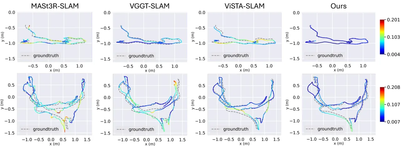
Figure 4: Qualitative trajectory comparison on 7-Scenes. UniSim-SLAM tracks the ground truth noticeably more closely than other feed-forward methods, especially on the chess sequence with its large depth variation.

The appendix extends the evaluation to Replica: an average ATE of 0.029 m over 8 sequences, against 0.072 for MASt3R-SLAM*, 0.042 for VGGT-SLAM and 0.108 for ViSTA-SLAM. Failure cases such as ViSTA-SLAM blowing up to 0.193 on office1 come out at 0.018 with UniSim-SLAM.

2. 3D Reconstruction: Accuracy and Chamfer Both Improve

Reconstruction uses the optimized global poses $\{T_i\}$ together with multi-view depths $\hat{D}^{\mathrm{mv}}$, intrinsics and confidence maps, discarding the lowest-confidence 25% of points following VGGT-SLAM. There is an honest evaluation detail here: because the framework produces overlapping submaps, stacking all points would artificially improve the Completeness metric simply through higher point density, so the authors take, for each view, the depth map of the single highest-confidence submap.

Method	Calib.	Acc. (lower better)	Comp. (lower better)	Chamfer (lower better)
DROID-SLAM	Calib.	0.111	0.049	0.080
MASt3R-SLAM	Calib.	0.064	0.068	0.066
Spann3R @5	Calib.	0.095	0.041	0.068
SLAM3R	Calib.	0.069	0.153	0.111
MASt3R-SLAM	UnCalib.	0.054	0.048	0.051
VGGT-SLAM	UnCalib.	0.039	0.051	0.045
ViSTA-SLAM	UnCalib.	0.041	0.056	0.049
UniSim-SLAM	UnCalib.	0.035	0.046	0.041

Table 3: 7-Scenes reconstruction error (Accuracy / Completeness / Chamfer, lower is better). UniSim-SLAM wins all three, and its Accuracy and Chamfer even beat every calibrated method.

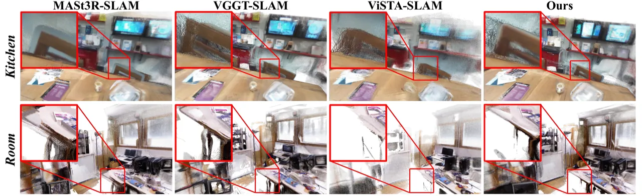
Figure 5: Reconstruction results on 7-Scenes and TUM RGB-D; red boxes mark zoomed-in detail views.

3. Latency: 197 ms in Exchange for 0.020 m

The authors define latency as the time "from receiving the minimum required input frames to the frontend producing a pose estimate". This table shows most clearly how the trade-off named in the title is resolved: VGGT-SLAM is decently accurate but takes 3410 ms, the purely two-view ViSTA-SLAM needs only 35 ms yet lands at 0.049 m error, and UniSim-SLAM buys 0.020 m for 197 ms. The heterogeneous "Ours + STA" variant is even more extreme: 35 ms latency with 0.027 m accuracy, cutting the error by 45% under exactly the same latency budget as ViSTA-SLAM.

Method	Frontend backbone	Latency [ms], lower better	ATE, lower better
MASt3R-SLAM	MASt3R	90	0.068
VGGT-SLAM	VGGT	3410	0.037
ViSTA-SLAM	STA	35	0.049
Ours + STA	STA	35	0.027
Ours	VGGT	197	0.020

Table 4: Latency versus accuracy on 7-Scenes. Higher latency does not imply higher accuracy: VGGT-SLAM spends 17x the time and is still less accurate than the 197 ms UniSim-SLAM.

Stage	Two-view inference (frontend)	Submap node init	Descriptor extraction	Graph construction	Optimization	Multi-view inference (backend)
Latency [ms]	197	167	16	36	645	933

Table 5: Per-stage timing breakdown (Appendix Table A6). The backend multi-view inference (933 ms) and graph optimization (645 ms) dominate, but they run on a separate thread and fire only once every 14 new keyframes, so they are not charged to frontend tracking latency.

4. Ablations: Every Edge Pulls Its Weight

Ablations are run on 7-Scenes and deliberately split into a "submap overlap $\phi=2$" and a "no overlap at all $\phi=0$" setting, the latter being exactly the failure scenario for multi-view methods that the paper keeps emphasizing.

Config	w/o Backend	w/o LC	w/o $\mathbf{e}^{\text{2v}}$	w/o $\mathbf{e}^{\mathrm{anch}}$	w/o $\mathbf{e}^{\mathrm{br}}$	w/o $\mathbf{e}^{\mathrm{tie}}$	w/o $\mathbf{e}^{\mathrm{sc}}$	Ours (full)
$\phi=0$	0.124	0.061	0.101	0.083	0.116	0.040	0.048	0.032
$\phi=2$	0.124	0.037	0.021	0.020	0.063	0.027	0.031	0.020

Table 6: Ablation of the 7-Scenes average ATE (lower is better). LC = loop closure.

Three conclusions deserve to be pulled out. First, the backend itself is the main source of gain: removing it (leaving frontend tracking only) gives 0.124 on average versus 0.020 for the full system, more than a sixfold difference. Second, the bridge edge $\mathbf{e}^{\mathrm{br}}$ is the single most important one: removing it degrades to 0.063 at $\phi=2$ (over three times worse) and to 0.116 at $\phi=0$, essentially back to tracking-only behaviour, which matches the explanation in Appendix A2: deleting view-to-submap edges disconnects submaps from the global trajectory, so global pose nodes are no longer constrained by submap predictions and the system degenerates into pure tracking without backend refinement. Third, the role of temporal edges is amplified when submaps do not overlap: at $\phi=0$, removing $\mathbf{e}^{\text{2v}}$ worsens 0.032 to 0.101, while at $\phi=2$ the change is only 0.020 to 0.021. Without submap overlap the temporal backbone is the sole channel through which corrections travel across the trajectory.

In addition, even with loop closure switched off entirely (0.037 at $\phi=2$) the system remains on par with existing state of the art, which shows that the graph itself already produces globally consistent optimization and that loop closure is the cherry on top.

Submap size $w$	$\phi=1$	$\phi=2$	$\phi=4$	$\phi=8$
4	0.043	0.041	-	-
8	0.035	0.035	0.035	-
16	0.031	0.032	0.031	0.030
32	0.033	0.032	0.034	0.033

Table 7: Hyperparameter sweep over submap size $w$ and overlap $\phi$ on TUM RGB-D (ATE RMSE [m]).

With only one frame of overlap ($\phi=1$), submap alignment relies entirely on a single multi-view local pose estimate and risks unstable optimization, so the default is $\phi=2$: robustness for minimal overhead. Submap size is a compromise, since a larger submap improves the local multi-view estimate but reduces the number of submap nodes in the graph and thus weakens global constraints, which is why $w=32$ is no better than $w=16$.

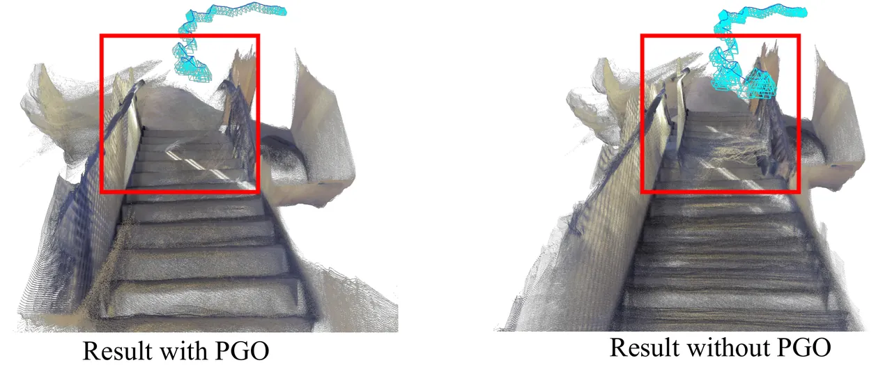
Figure 6: Qualitative comparison with and without pose graph optimization (PGO), from paper Fig. A1. Red boxes mark misaligned regions corrected by PGO.

5. Robustness of the Scale Anchor

Since the whole method puts a 50x weight on a scale estimated from depth statistics, a natural objection is whether that anchor stays put when the depth is noisy. The authors run a controlled experiment injecting noise of different standard deviations $\sigma$ into the depth used for scale estimation and into the depth used for geometry, separately.

Perturbation target	Depth noise $\sigma$	7-Scenes average ATE
Scale	0.15	0.045
	0.1	0.041
	0.05	0.026
	0	0.020
Depth	0.3	0.021
	0.2	0.021
	0.1	0.020
	0	0.020

Table 8: Robustness of the depth-statistic scale estimation (Appendix Table A3). Noise applied directly to the scale estimate degrades results clearly (0.020 to 0.045 at $\sigma=0.15$), whereas noise applied to the dense depth barely matters (still 0.021 at $\sigma=0.3$).

The asymmetry is informative: a median statistic is almost immune to random noise on a dense depth map, since it takes the median of thousands of per-pixel ratios, but if the noise lands precisely on the depths participating in scale estimation the anchor is biased systematically. This also explains why $w^{\text{anch}}$ and $w^{\text{sc}}$ are set to 50: the scale constraint has to be strong, but its quality ceiling is set by the reliability of the depth ratio.

Limitations

Stated by the authors: latency is still higher than a dedicated two-view pipeline. The 197 ms tracking latency of UniSim-SLAM is far below the 3410 ms of VGGT-SLAM but above both MASt3R-SLAM (90 ms) and ViSTA-SLAM (35 ms). The authors attribute this to the large model size of the VGGT frontend backbone and its general-purpose design. In other words, the accuracy-efficiency trade-off is mitigated, not eliminated; applications with a very tight latency budget have to fall back to the heterogeneous "Ours + STA" configuration at 35 ms, paying with accuracy dropping from 0.020 to 0.027 and inheriting the intrinsic weaknesses of STA-based SLAM on hard sequences such as chess and plant.

Stated by the authors: the backend is not cheap. The breakdown in Table 5 shows one backend pass costs 933 ms of multi-view inference plus 645 ms of graph optimization, on top of 167 ms for submap node initialization. Although the asynchronous thread hides this from the frontend, it raises the practical question of whether backend refinement can keep up with keyframe production on compute-constrained embedded platforms; the paper offers no analysis of behaviour under a backend backlog.

Additional observations from the reader's side. First, accuracy visibly drops when submaps do not overlap: the average ATE is 0.032 at $\phi=0$ versus 0.020 at $\phi=2$, a 60% degradation. The paper sells "corrections still propagate through temporal edges even without overlap", but the numbers show the method still benefits substantially from submap overlap; in a purely non-overlapping scenario (fast turns or long straight stretches) performance is merely usable rather than excellent. Second, dense reconstruction is evaluated only on 7-Scenes, with TUM RGB-D limited to qualitative figures, while TUM's large planar scenes such as floor and room are exactly where scale is hardest to recover, leaving reconstruction quality there unknown. Third, scale anchoring relies on the comparability of two-view and multi-view depth; with a heterogeneous frontend/backend pair (STA + VGGT) the two models follow different depth conventions and scale biases, weakening the statistical meaning of $\mathrm{median}(\hat{D}^{\mathrm{mv}}/\hat{D}^{\text{2v}})$. The paper validates the heterogeneous configuration only at the level of pose accuracy and never analyses scale anchoring quality in isolation. Fourth, the code is not public, so none of the numbers above can currently be reproduced. Fifth, loop closure depends on the SALAD descriptor retrieval threshold and on VGGT geometric verification, yet the paper reports neither loop recall nor precision, and gives no analysis of false-loop risk under perceptual aliasing.

Conclusion and Outlook

The contribution of this paper is not a new geometric foundation model but a clean answer to the question of how to organize the outputs of feed-forward models into a SLAM system: accept that feed-forward predictions are configuration-dependent, heterogeneous and scale-inconsistent, then do not try to force them into one coordinate frame; instead build a multi-level factor graph on $Sim(3)$ and let different types of prediction coexist as constraints at different levels and weights, optimized jointly. The perspective transfers well. It explains why the classical frontend/backend division of labour still holds in the feed-forward era, and it names the concrete reason naive concatenation fails: a degenerate solution exists, because submap alignment can be compensated by displacing intermediate view nodes, so direct submap-to-submap edges are mandatory.

The two numbers worth remembering from an engineering standpoint are the stability bought by boosting the scale constraint weight 50x, and the fact that under an identical 35 ms latency budget the multi-level factor graph drives ViSTA-SLAM's 0.049 m down to 0.027 m. The latter shows that this graph optimization can be grafted onto existing low-latency two-view systems as a backend upgrade without replacing the whole system. The natural next steps are to bring down the backend cost of multi-view inference and graph optimization (933 + 645 ms is the current bottleneck) and to validate on dynamic scenes, large-scale outdoor sequences and embedded compute, none of which the present evaluation (static indoor scenes, a few thousand frames) covers.

Golden Quote

A feed-forward model never returns "one answer"; it returns many locally valid answers whose scales disagree. The job of SLAM is not to pick the best one but to give them a graph in which they can all hold at once.