DL-SLAM: Enabling High-Fidelity Gaussian Splatting SLAM in Dynamic Environments based on Dual-Level Probability

Paper Metadata

• Title: DL-SLAM: Enabling High-Fidelity Gaussian Splatting SLAM in Dynamic Environments based on Dual-Level Probability
• Authors: Ziheng Xu, Qingfeng Li, Xuefeng Liu, Chen Chen, Jianwei Niu (the same group previously published NID-SLAM and has worked on dense SLAM in dynamic environments for several years)
• Venue: ACM Multimedia 2026 (Rio de Janeiro); arXiv 2607.01860v2 [cs.RO]
• Link: arxiv.org/abs/2607.01860
• Code status: No official repository was found as of this writing (GitHub search returns no matching project), and the paper lists no code link

One-Sentence Summary

DL-SLAM equips Gaussian Splatting SLAM with a dual-level dynamic-probability framework — pixel-level probabilities weight tracking, object-level probabilities drive categorical pruning of dynamic Gaussians — so that transiently static objects help localize the camera without ever contaminating the static map, yielding state-of-the-art tracking and artifact-free rendering on TUM RGB-D, BONN, and Wild-SLAM iPhone.

Background and Motivation

Visual SLAM underpins embodied AI, autonomous driving, and mixed reality. The latest generation of dense SLAM systems, built on Neural Radiance Fields or 3D Gaussian Splatting (3DGS), delivers novel-view synthesis and high-fidelity mapping that classical methods could not approach. But nearly all of these systems inherit the static-world assumption. When people walk through the frame or boxes are carried across the room, moving objects inject false inter-frame correspondences that corrupt camera pose estimation, and any dynamic geometry that leaks into the map becomes a persistent visual artifact. Reconciling dynamic scenes with high-fidelity reconstruction is one of the gating problems for dense SLAM in real deployments.

The dominant remedy so far has been blunt: use a semantic segmentation network to identify predefined dynamic categories — persons, cars — and exclude those masked regions from tracking and mapping entirely. DynaSLAM, DG-SLAM, and SDD-SLAM all follow this recipe. The paper identifies two structural flaws in it. First, dynamic objects are not always harmful. When they are transiently static — a person standing still, a cart parked mid-corridor — they provide valuable geometric and photometric constraints for pose estimation. Throwing those pixels away indiscriminately is actively counterproductive when dynamic objects dominate the image, because the remaining static structure is then too sparse to constrain the camera at all. Second, a fixed category list bounds generalization: any moving object outside the predefined classes (a sliding chair, a transported box) is silently treated as static background.

WildGS-SLAM, the closest predecessor, tried to recover that lost information by estimating per-pixel uncertainty maps and using them as weights during tracking, so transiently static objects can contribute to pose estimation. The paper's analysis attributes two weaknesses to it. One: because low-uncertainty regions are treated as trustworthy, transiently static objects get fused into the map representation, leaving persistent artifacts — an object that merely paused is enshrined as permanent scenery. Two: the uncertainty estimate is purely geometric, so it becomes ambiguous right at object boundaries, precisely where dynamic-region identification matters most.

DL-SLAM's design goal can be stated in one line: let transiently static objects help tracking, but never let them enter the map. Achieving both in a single system requires reasoning at two granularities. Pixel-level judgments are fine-grained enough for per-residual weighting, yet they cannot see an object's global motion state; object-level judgments can declare an instance dynamic, yet they are only as reliable as the pixel evidence feeding them. The paper's answer is a dual-level probabilistic framework. Pixel-level dynamic probabilities are computed from semantic and geometric cues and serve as adaptive weights in dense bundle adjustment (DBA). These probabilities are lifted into per-Gaussian attributes and aggregated per instance into object-level probabilities, which gate categorical pruning. The purified static map is then rendered back into a geometrically consistent probability map that Bayesian-updates the pixel-level estimates — closing the loop between the two levels.

A fourth, less advertised contribution targets semantic mapping quality under dynamics. Object motion and heavy occlusion make per-frame semantic labels temporally inconsistent and spatially hollow. DL-SLAM adds a dynamic-aware semantic refinement strategy that merges inconsistent labels online and densifies occluded regions, which is what ultimately supports an object-level semantic map you can edit interactively. Together these pieces form the complete ACM MM 2026 story.

Preliminaries: A 3DGS Representation Extended with Dynamic Probability

The static part of the scanned environment is represented by a set of anisotropic 3D Gaussians $\mathcal{G}=\{g_i\}_{i=1}^{K}$. Each Gaussian $g_i$ carries a mean $\mu_i\in\mathbb{R}^3$, covariance $\Sigma_i\in\mathbb{R}^{3\times3}$, opacity $o_i\in[0,1]$, and RGB color $c_i\in\mathbb{R}^3$. DL-SLAM adds two attributes to every Gaussian: a dynamic probability $p_i\in[0,1]$ and an explicit semantic label $\ell_i$. The probability is a continuous score where higher values indicate a greater likelihood of motion; the explicit label follows the OpenGS-SLAM paradigm of attaching discrete class identities to Gaussians, which enables direct object-level reasoning instead of the decoding stage that implicit feature vectors require.

Rendering uses standard alpha-blending. The color image $\hat{C}$ and depth map $\hat{D}$ are:

$$\hat{C}=\sum_{i=1}^{n} c_i \alpha_i T_i,\qquad \hat{D}=\sum_{i=1}^{n} d_i \alpha_i T_i,\qquad T_i=\prod_{j=1}^{i-1}(1-\alpha_j) \tag{1}$$

where $c_i$ and $d_i$ are the color and depth of Gaussian $g_i$, and the transmittance $T_i$ is the fraction of light that reaches Gaussian $i$ without being absorbed by predecessors. The opacity of the splatted 2D Gaussian in pixel space is:

$$\alpha_i=o_i\exp\left(-\frac{1}{2}(u-\mu)^{T}\Sigma_{2D}^{-1}(u-\mu)\right) \tag{2}$$

with pixel coordinate $u$ and the projected 2D mean and covariance $\mu$, $\Sigma_{2D}$. The deceptively simple move is that the dynamic probability map is rendered exactly like color and depth:

$$\hat{P}=\sum_{i=1}^{n} p_i \alpha_i T_i \tag{3}$$

This single equation is the substrate of the feedback loop: it lets the system render a geometrically consistent probability map from the 3D map, rather than relying solely on frame-to-frame 2D estimates. The semantic label map $\hat{L}$ is rendered by Gaussian voting: the cumulative weight of label $l_j$ is

$$W_j=\sum_{g_i\in\mathcal{G}_j^{u}}\alpha_i\prod_{k=1}^{i-1}(1-\alpha_k) \tag{4}$$

where $\mathcal{G}_j^{u}$ is the set of Gaussians contributing to pixel $u$ with label $l_j$; the label with the highest weight wins the pixel.

Method in Detail

Figure 2 shows the system overview. From an RGB sequence, the tracking branch estimates a pixel-level dynamic probability map $P$ and feeds it into DBA as per-pixel weights; the mapping branch lifts probabilities and labels into the Gaussian representation, performs object-level probability estimation and dynamic pruning; the purified static map then renders a probability map $\hat{P}'$ that refines the pixel-level estimates. Each stage below follows that data flow.

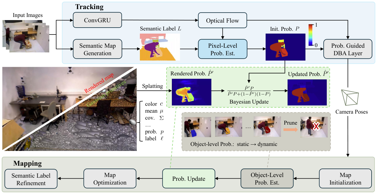
Figure 2: System overview (paper Fig. 2). Tracking uses the semantic label map and optical flow to estimate a pixel-level dynamic probability map that weights DBA. Mapping lifts probabilities and labels into Gaussian attributes for object-level estimation and pruning; the static map renders a probability map that Bayesian-updates the initial pixel-level estimate.

Semantic Map Generation: Open-Vocabulary Segmentation with Cross-Frame Association

The foundation of the framework is robust, temporally consistent scene semantics. Rather than depending on predefined dynamic categories such as "person", DL-SLAM goes open-vocabulary: the Recognize Anything Model (RAM) produces open-set class tags from the input image; those tags act as text prompts for Grounding DINO, which outputs class-aware bounding boxes; MobileSAMv2 then produces fine-grained semantic label maps. Because nothing in this chain assumes a fixed list of dynamic classes, any detected instance can enter the probabilistic reasoning downstream.

Per-frame segmentation alone is insufficient — labels must be associated to stable instance identities across frames. OpenGS-SLAM matched detections by IoU alone, which breaks down for dynamic objects with large displacements. DL-SLAM instead computes a fused matching score combining spatial overlap (IoU) and appearance similarity measured with CLIP features. Each new detection is scored against all tracked objects of the same class; the highest-scoring object above threshold $\tau_{sim}=0.7$ donates its identity, and unmatched detections initialize new labels. The result is a semantic label map $L$ in which every object keeps a consistent ID across frames — a precondition for any object-level probability aggregation.

Pixel-Level Dynamic Probability: Statistical Modeling of Epipolar Error

The pixel-level question is: under the static-scene hypothesis, how inconsistent is this pixel's observation? DL-SLAM quantifies inconsistency with epipolar geometry. For efficiency, probability maps are estimated only on keyframes: a ConvGRU network estimates optical flow between the current keyframe $I_k$ and the previous keyframe $I_{k-1}$ (the same flow also serves pose estimation), a fundamental matrix $F_{k,k-1}$ is estimated from the dense flow correspondences, and each pixel $u$ receives a Sampson error $e_{F_{k,k-1}}(u)$ measuring its deviation from the epipolar constraint.

The geometric error is then given a statistical interpretation, inspired by CFP-SLAM: assuming the error of static pixels is Gaussian-distributed, the squared Sampson error follows a chi-squared distribution with two degrees of freedom. The dynamic probability of pixel $u$ is the CDF of that distribution:

$$\tilde{P}_{k|k-1}(u)=\mathrm{CDF}_{\chi^2}\left(\left(e_{F_{k,k-1}}(u)\right)^{2};\,2\right) \tag{5}$$

Larger geometric error translates directly into higher dynamic likelihood. Compared with WildGS-SLAM, which optimizes an uncertainty-estimation network online, this analytic construction is nearly free, and the semantic masks supply the boundary priors that pure geometry lacks.

The initial map $\tilde{P}_{k|k-1}$ is then semantically aggregated. The rigid-object assumption says all pixels on one object share a motion state. For each object $o$, the per-pixel probabilities inside its mask $\mathcal{M}_o$ are collected and sorted in descending order; the object's 2D dynamic probability $p^{2D}_o$ is the average of the first quartile and the median, and that value is assigned to every pixel in the mask to form the aggregated map $P_k$. This "significant motion dictates the object state" rule is robust to isolated noisy pixels while refusing to let a majority of static readings dilute genuine motion.

Object-Level Dynamic Probability: Recency-Weighted Aggregation

Pixel-level information is lifted into 3D at Gaussian creation time: every new Gaussian $g_i$ spawned from keyframe $k$ inherits dynamic probability $p_i$ and semantic label $\ell_i$ from its source pixel. The naive object-level probability — a plain average over all of an object's Gaussians — suffers from temporal inertia: an object that was static for a long time accumulates a large stock of low-probability Gaussians, so when it finally starts moving, fresh high-probability Gaussians are diluted by history and the system reacts late.

DL-SLAM counters with recency-weighted aggregation. Let $\mathcal{G}_o$ be the Gaussians of object $o$. At keyframe $k$, each Gaussian receives an exponentially decaying weight $w_i=\exp(-\delta(k-k_i))$, where $k_i$ is the creation keyframe index of $g_i$ and $\delta=0.3$ is the decay rate. The object-level probability is the weighted mean:

$$p^{3D}_o=\frac{\sum_{g_i\in\mathcal{G}_o}w_i p_i}{\sum_{g_i\in\mathcal{G}_o}w_i} \tag{6}$$

Recent behavior now dominates the motion state, so state changes are detected quickly. The design rhymes with the pixel-level quartile aggregation: both levels answer the same question — how to make motion that is happening now outweigh stillness that used to be.

Temporal Confirmation and Categorical Pruning

Pruning is deliberately conservative to avoid deleting static objects prematurely. An object is declared dynamic and added to a global dynamic set only if its $p^{3D}_o$ exceeds $\tau_{prune}=0.8$ for three consecutive keyframes; all Gaussians belonging to any object in that set are then removed from the scene. The three-frame confirmation trades a little reaction speed for robustness against transient misjudgments. Once confirmed, removal is categorical and instance-wide — this is the direct source of the artifact-free static map, and it is precisely where DL-SLAM departs from WildGS-SLAM's "low uncertainty means fuse it into the map" behavior.

Probability Update: A Bayesian Feedback Loop Through the Static Map

The fidelity of the aggregated map $P_k$ is bounded by the reliability of the initial estimate $\tilde{P}_{k|k-1}$, and 2D optical-flow-based estimates err in textureless regions. Classical geometry-based pipelines such as CFP-SLAM update probabilities through costly multi-stage procedures; DL-SLAM does it through the 3D representation itself. The map renders a geometrically consistent probability map $\hat{P}_k$ via Eq. (3). Because rendering is a weighted average, high-probability dynamic Gaussians get diluted among many static ones, so the rendered map is amplified by power-law scaling $\hat{P}'_k=(\hat{P}_k)^{\gamma}$ with $\gamma=0.5$, then fused with the initial estimate in a Bayesian update:

$$P^{post}_k=\frac{\hat{P}'_k\cdot P_k}{\hat{P}'_k\cdot P_k+(1-\hat{P}'_k)\cdot(1-P_k)} \tag{7}$$

The expression multiplies the map-rendered likelihood with the frame-to-frame prior and renormalizes: pixels that both sources consider dynamic are pushed up, and a strong static vote from either side pulls the posterior down. The 2D posterior is then propagated back into 3D: all visible Gaussian centers are projected onto the image plane at the current viewpoint, and each Gaussian's dynamic attribute $p_i$ is overwritten with the corresponding pixel posterior. Pixel level and object level have now exchanged information through the 3D map — the true meaning of "dual-level" coupling in the title.

Dynamic-Aware Semantic Label Refinement

Semantic mapping under dynamics faces two challenges. First, despite 2D data association, label inconsistencies persist because frame-to-frame matching lacks the global geometric context of the 3D map. Second, moving objects occlude regions that end up sparse and under-reconstructed, populated by semantically ambiguous Gaussians. For the first problem, the paper introduces an online correction mechanism that decides whether a rendered mask $\mathcal{M}_i\subset\hat{L}$ with label $i$ and an input mask $\mathcal{M}_j\subset L$ with label $j$ correspond to the same object, using a score that takes the maximum of IoU and both containment ratios:

$$S_m(i,j)=\max\left(\frac{|\mathcal{M}_i\cap\mathcal{M}_j|}{|\mathcal{M}_i\cup\mathcal{M}_j|},\frac{|\mathcal{M}_i\cap\mathcal{M}_j|}{|\mathcal{M}_j|},\frac{|\mathcal{M}_i\cap\mathcal{M}_j|}{|\mathcal{M}_i|}\right) \tag{8}$$

When $S_m(i,j)$ exceeds $\tau_{match}=0.8$, label $j$ is considered an alias of label $i$. To resist transient errors, the association must repeat for three consecutive keyframes before it solidifies into a permanent identity merge, after which the affected Gaussians are relabeled. Including containment ratios lets the matcher succeed in occlusion scenarios where the rendered mask covers only part of the input mask. For the second problem, semantic fragmentation is measured by a pixel-wise semantic gradient:

$$S_g(u)=\sum_{q\in\mathcal{N}(u)}\mathbb{1}\left(\hat{L}(u)\neq\hat{L}(q)\right) \tag{9}$$

where $\mathcal{N}(u)$ is the 4-connected neighborhood of $u$ and $\mathbb{1}(\cdot)$ is the indicator function. Inside the union of all dynamic object masks, regions where $S_g(u)$ exceeds $\tau_{grad}=3$ are targeted for densification, completing reconstruction holes left by occluding objects. Figure 3 shows the effect.

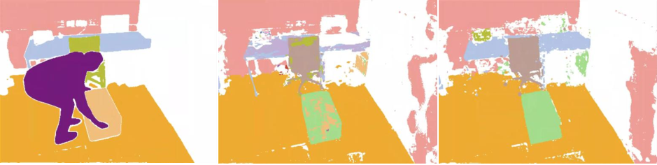
Figure 3: Effect of semantic label refinement (paper Fig. 3, Bonn_mv_box2, frame 520). Left to right: input label map, rendering without refinement, rendering with refinement. The method resolves semantic inconsistencies (e.g., the box on the floor) and robustly reconstructs regions occluded by dynamic objects (e.g., the chair).

Tracking and Mapping: Probability-Weighted DBA and Local Window Optimization

The tracker builds on DROID-SLAM: a DBA layer jointly optimizes keyframe poses $\omega$ and disparities $d$ over a frame graph $\mathcal{F}=(V,E)$. DL-SLAM estimates metric depth $\tilde{D}_i$ for every new keyframe with Metric3D and injects the dynamic probability map into the DBA objective as weights:

$$\arg\min_{\omega,d}\sum_{(i,j)\in E}\left\|\tilde{u}_{ij}-\Pi_c\left(\omega_j^{-1}\omega_i\Pi_c^{-1}(u_i,d_i)\right)\right\|^{2}_{\Sigma_{ij}/(1-P_i)} \tag{10}$$

Here $u_i$ are pixel coordinates of keyframe $I_i$, $\tilde{u}_{ij}$ is the optical-flow-predicted correspondence with keyframe $I_j$, $\Pi_c$ is the camera projection function, and the information matrix combines the ConvGRU confidence $\Sigma_{ij}$ with the dynamic probability $P_i$. Because the weight is $\Sigma_{ij}/(1-P_i)$, pixels whose dynamic probability approaches one contribute vanishingly little: actively moving pixels are down-weighted, while stable regions of transiently static objects keep constraining the solution. That is the concrete mechanism by which transient objects "help tracking".

On the mapping side, the Gaussian map grows incrementally with new keyframes. Unlike methods that filter dynamic objects in 2D, DL-SLAM lets every pixel initialize new Gaussians and defers all dynamic handling to 3D pruning, so a 2D misjudgment never irreversibly destroys information. After expansion, the map is optimized over a local window of covisible keyframes with the rendering loss:

$$(1-P)\left(\lambda_c\mathcal{L}_{color}+(1-\lambda_c)\mathcal{L}_{depth}\right)+\lambda_{reg}\mathcal{L}_{iso} \tag{11}$$

Both the color and depth terms are weighted by $(1-P)$, so dynamic pixels provide no supervision. The color loss blends L1 and SSIM:

$$\mathcal{L}_{color}=(1-\lambda_{ssim})|\hat{C}-C|_1+\lambda_{ssim}\left(1-\mathrm{SSIM}(\hat{C},C)\right) \tag{12}$$

The depth loss $\mathcal{L}_{depth}=|\hat{D}-\tilde{D}|_1$ supervises rendering against Metric3D metric depth. An isotropic regularizer prevents Gaussians in weakly constrained regions from elongating:

$$\mathcal{L}_{reg}=\frac{1}{|\mathcal{G}|}\sum_{i=1}^{|\mathcal{G}|}|s_i-\bar{s}_i|_1 \tag{14}$$

where $s_i$ is the scale of the $i$-th Gaussian and $\bar{s}_i$ the mean scale in the map. One more engineering detail: instead of a fixed iteration count, optimization terminates when the variance of the mapping loss across the local window drops below $\tau_{var}=0.002$, skipping redundant iterations after convergence. The implementation uses $\lambda_c=0.5$, $\lambda_{reg}=10$, $\lambda_{ssim}=0.2$.

flowchart TD
    A[RGB keyframe sequence] --> B[Open-vocabulary segmentation
RAM + Grounding DINO + MobileSAMv2]
    B --> C[Cross-frame data association
IoU + CLIP appearance similarity]
    C --> D[Semantic label map L
consistent instance IDs]
    A --> E[ConvGRU optical flow]
    E --> F[Fundamental matrix and Sampson error]
    F --> G[Pixel-level initial probability
chi-square CDF model]
    D --> H[Per-object semantic aggregation
first quartile plus median]
    G --> H
    H --> I[Aggregated map P weights DBA tracking
dynamic pixels down-weighted]
    H --> J[Lift probability and label
into Gaussian attributes]
    J --> K[Object-level probability
recency-weighted aggregation]
    K --> L{Above 0.8 for three
consecutive keyframes}
    L -->|yes| M[Categorical pruning of dynamic Gaussians]
    M --> N[Purified static map]
    N --> O[Render probability map
power-law scaling]
    O --> Q[Bayesian posterior update
of pixel probabilities]
    Q --> H
    D --> R[Semantic label correction
and occlusion-aware densification]
    R --> N

The DL-SLAM dual-level pipeline: pixel-level probabilities weight tracking, object-level probabilities drive pruning, and the static map's rendered probability feeds back through a Bayesian update to close the loop.

Experiments

All experiments run on a desktop with an Intel i9-12900KF CPU and an NVIDIA RTX 3090 GPU. Evaluation spans three dynamic benchmarks: the TUM RGB-D dynamic subset (8 sequences), BONN (8 sequences), and the Wild-SLAM iPhone dataset (piano, shop, street, tower, wall, wander) for unconstrained settings. Tracking accuracy is measured by ATE RMSE and standard deviation; reconstruction and rendering quality by PSNR, SSIM, and LPIPS against ground-truth training views. Baselines are grouped by scene representation: traditional (ORB-SLAM2, ReFusion, DynaSLAM, CFP-SLAM), NeRF-based (Co-SLAM, NID-SLAM, RoDyn-SLAM, DynaMoN), and 3DGS-based (SGS-SLAM, DG-SLAM, SDD-SLAM, WildGS-SLAM), each group including one static method as reference.

Tracking: First Place on Both TUM and BONN

Table 1 reports tracking on TUM RGB-D (ATE RMSE in cm). DL-SLAM is best on six of the eight sequences and ties or nearly ties on the rest, with an average RMSE of 1.3 cm — about 13% lower than the runner-up WildGS-SLAM (1.5 cm). That is the source of the abstract's "up to 13% tracking improvement". The semantic-mask family (DynaSLAM, CFP-SLAM) averages 1.7–1.9 cm, while static methods that ignore dynamics collapse on the high-dynamic walk sequences: ORB-SLAM2 averages 30.2 cm and Co-SLAM 63.3 cm, with individual sequences exceeding two meters.

Method	f3/sit_s	f3/sit_x	f3/sit_r	f3/sit_h	f3/walk_s	f3/walk_x	f3/walk_r	f3/walk_h	Avg.
ORB-SLAM2	0.9	0.9	2.0	1.9	38.7	72.1	78.4	46.7	30.2
ReFusion	0.9	4.0	13.2	11.0	1.7	9.9	40.6	10.4	11.5
DynaSLAM	0.5	1.3	2.7	1.9	0.7	1.6	3.5	3.0	1.9
CFP-SLAM	0.5	0.9	2.5	1.5	0.7	1.4	3.7	2.4	1.7
Co-SLAM	1.5	4.8	51.7	8.6	30.6	72.5	236.0	100.7	63.3
NID-SLAM	1.9	7.5	8.6	10.5	6.2	6.4	64.8	7.1	14.1
RoDyn-SLAM	1.7	5.2	6.7	4.4	1.7	8.3	7.9	5.6	5.2
DynaMoN	0.5	1.0	2.4	2.6	0.7	1.4	3.5	1.9	1.8
SGS-SLAM	1.4	1.8	13.5	12.9	60.3	130.4	70.7	69.6	37.2
DG-SLAM	0.7	1.1	3.6	2.5	3.5	2.9	4.4	3.7	2.8
WildGS-SLAM	0.5	0.8	2.3	1.7	0.5	1.3	3.1	1.5	1.5
DL-SLAM (Ours)	0.5	0.8	1.9	1.3	0.4	1.2	2.9	1.4	1.3

Table 1: Tracking on TUM RGB-D dynamic, ATE RMSE [cm], lower is better (paper Table 3; standard deviations omitted here). Bold marks column-best.

BONN (Table 2) shows the same ordering: DL-SLAM averages 2.2 cm RMSE versus 2.5 cm for WildGS-SLAM, a roughly 12% margin, with the clearest wins in the crowded sequences (crowd: 1.3 vs 1.6 cm; crowd2: 1.6 vs 2.2 cm). Two honest exceptions: on ps_trk2, DynaMoN edges ahead (2.3 vs 2.9 cm), and on mv_box2, WildGS-SLAM is best (2.3 vs 2.6 cm). 3DGS-based methods occupy the entire top tier, while static methods average 22–90 cm on BONN — another demonstration that dynamic handling is not optional.

Method	ball	ball2	crowd	crowd2	ps_trk	ps_trk2	mv_box	mv_box2	Avg.
ORB-SLAM2	15.8	12.6	98.0	62.8	69.8	78.6	32.3	79.6	56.2
DynaSLAM	3.4	3.2	2.5	2.9	4.7	12.6	2.0	26.2	7.2
Co-SLAM	25.0	38.7	245.8	229.0	77.2	73.7	10.5	25.4	90.7
RoDyn-SLAM	7.9	11.5	13.5	13.7	14.5	13.8	24.9	12.6	14.1
DynaMoN	2.9	2.7	3.3	4.8	15.1	2.3	1.5	2.7	4.4
SGS-SLAM	44.7	37.2	105.8	267.0	128.7	66.7	23.6	41.5	89.4
DG-SLAM	6.2	4.8	2.1	3.2	4.6	6.3	2.8	3.6	4.2
WildGS-SLAM	2.8	2.5	1.6	2.2	3.7	3.1	1.7	2.3	2.5
DL-SLAM (Ours)	2.4	2.3	1.3	1.6	3.4	2.9	1.4	2.6	2.2

Table 2: Tracking on BONN, ATE RMSE [cm] (excerpt of paper Table 2; ReFusion and SDD-SLAM omitted due to incomplete reporting). Bold marks column-best.

Rendering: Quantitative Evidence for an Artifact-Free Map

The rendering evaluation is the quantitative case for "pruning yields an artifact-free map". Table 3 gives the full Wild-SLAM iPhone results: DL-SLAM takes the best PSNR and SSIM on all six sequences — for instance, piano at 19.18 dB (WildGS-SLAM 17.93, SGS-SLAM 16.65), street at 21.06 dB (WildGS 19.69), and tower at 19.93 dB — plus the best LPIPS on five of six sequences. The paper's qualitative comparison (its Fig. 4) explains the gap: WildGS-SLAM fuses the two transiently static persons into the wandering map and leaves the moved box at its original location in mv_box, producing visible artifacts; DL-SLAM's object-level pruning removes those Gaussians entirely. The mv_box case is worth emphasizing: the box that travels from table to floor is correctly classified as dynamic and cleared from both its initial and final positions. On BONN, DL-SLAM likewise leads PSNR and SSIM on all eight sequences.

Method	Metric	piano	shop	street	tower	wall	wander
SGS-SLAM	PSNR [dB]↑	16.65	15.59	18.31	17.53	14.15	14.11
	SSIM↑	0.669	0.584	0.736	0.715	0.415	0.513
	LPIPS↓	0.409	0.583	0.418	0.385	0.681	0.561
DG-SLAM	PSNR [dB]↑	13.41	12.76	13.23	13.98	11.97	13.14
	SSIM↑	0.263	0.227	0.375	0.531	0.203	0.260
	LPIPS↓	0.846	0.936	0.855	0.674	0.994	0.831
WildGS-SLAM	PSNR [dB]↑	17.93	15.79	19.69	19.06	16.32	16.70
	SSIM↑	0.650	0.499	0.700	0.805	0.503	0.569
	LPIPS↓	0.248	0.468	0.337	0.245	0.493	0.341
DL-SLAM (Ours)	PSNR [dB]↑	19.18	18.34	21.06	19.93	18.07	17.92
	SSIM↑	0.764	0.689	0.810	0.864	0.715	0.751
	LPIPS↓	0.171	0.236	0.175	0.163	0.236	0.197

Table 3: Rendering on the Wild-SLAM iPhone dataset (excerpt of paper Table 1).

The object-level semantic map also unlocks a practical capability: interactive scene editing. In the paper's Fig. 5 (shown below), a user prompt names a target object in the iPhone tower sequence, the system locates the corresponding instance, and removes it from the final map.

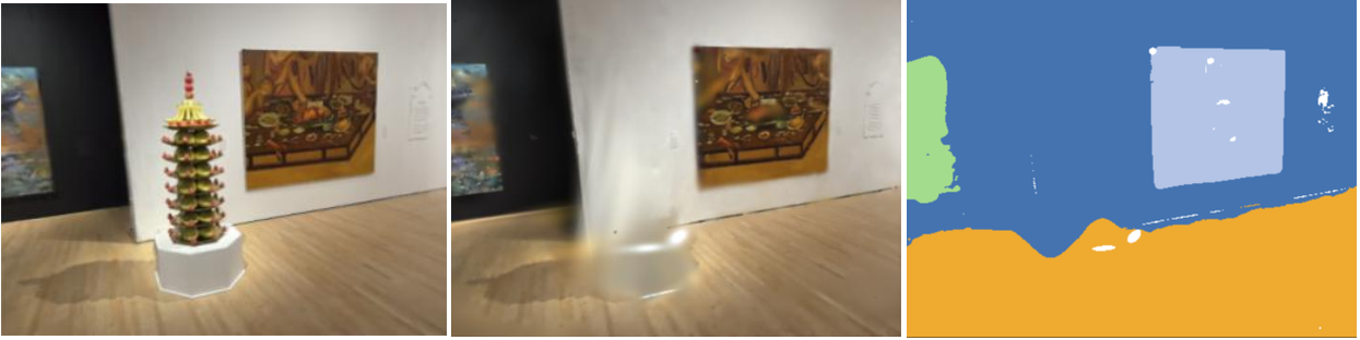
Figure 4: Interactive scene editing on Wild-SLAM iPhone (paper Fig. 5, tower sequence, frame 171). Left to right: rendering before removal, RGB rendering after removal, semantic rendering after removal. The target instance is specified by a user prompt.

Runtime, Memory, and Ablations

Table 4 reports runtime and memory on TUM RGB-D. Segmentation costs 168.5 ms/frame — SGS-SLAM is given the same labels for a fair comparison, so the two tie here. Tracking costs 139.6 ms/frame, tied with WildGS-SLAM for lowest thanks to the shared efficient DBA layer (SGS-SLAM spends 1307.1 ms/frame). Mapping costs 590.4 ms/frame, best among all compared methods; WildGS-SLAM's 995.9 ms reflects the online optimization of its uncertainty network. The model size is 11.1 MB, about three times more compact than SGS-SLAM's 32.9 MB, but GPU memory peaks at 11.5 GB — the highest in the comparison, a direct consequence of storing semantic labels and dynamic probabilities per Gaussian. The paper does not report an end-to-end FPS; summing the per-stage costs makes clear the system is not real-time.

Metric	RoDyn-SLAM	SGS-SLAM	WildGS-SLAM	DL-SLAM (Ours)
Segmentation [ms/frame]↓	250.0	168.5	–	168.5
Tracking [ms/frame]↓	378.4	1307.1	139.6	139.6
Mapping [ms/frame]↓	757.2	620.3	995.9	590.4
Model size [MB]↓	7.3	32.9	8.0	11.1
GPU memory [GB]↓	5.0	6.5	10.8	11.5

Table 4: Runtime and memory on TUM RGB-D (paper Table 4). Bold marks row-best; WildGS-SLAM has no separate segmentation module.

The ablation study (Table 5, averaged over the 8 BONN sequences) quantifies each component's contribution. Removing pixel-level probability is the most expensive change: ATE RMSE nearly doubles from 2.2 to 4.8 cm, confirming that probability-weighted DBA is the main driver of robust tracking. Removing object-level probability raises ATE to 2.6 cm and drops PSNR from 19.99 to 19.38 dB; the paper's qualitative results show visible ghosting of dynamic persons in the crowd2 sequence. Removing semantic refinement hurts rendering most, dropping PSNR to 18.74 dB. Each component earns its place: pixel-level protects tracking, object-level protects the map, semantic refinement protects rendering and label fidelity.

Configuration	ATE RMSE [cm]↓	ATE S.D. [cm]↓	PSNR [dB]↑
w/o pixel-level prob.	4.8	2.8	19.00
w/o object-level prob.	2.6	1.3	19.38
w/o semantic refinement	2.4	1.1	18.74
DL-SLAM (full)	2.2	1.0	19.99

Table 5: Ablation on BONN (paper Table 5).

Figure 5: Rendering ablation on BONN (paper Fig. 6, crowd2, frame 316). Left to right: ground truth, rendering without object-level probability, full DL-SLAM rendering, and a zoomed-in view. Without object-level pruning, dynamic persons remain in the map as ghosting artifacts.

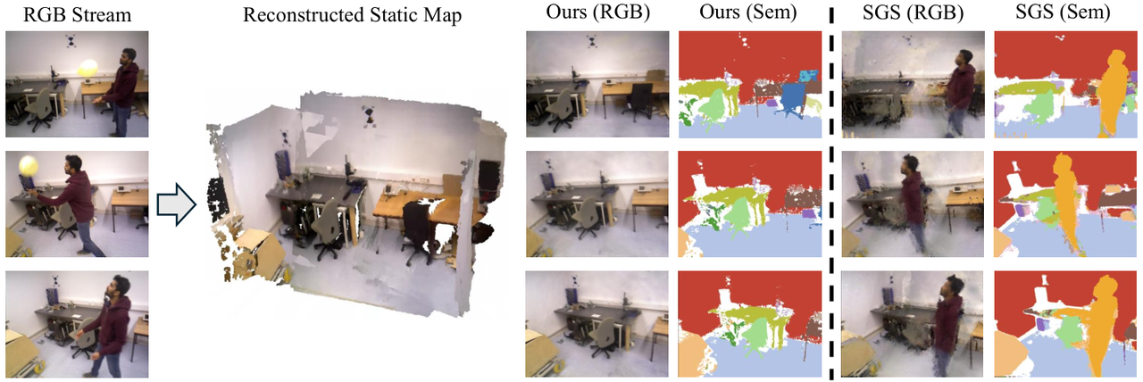
Figure 6: Paper teaser (Fig. 1). Static-map reconstruction from a monocular dynamic sequence: DL-SLAM eliminates dynamic-object interference in both RGB and semantic views, whereas SGS-SLAM retains heavy ghosting.

Limitations

1. Only the static scene is modeled; dynamic objects are discarded rather than understood (author-stated). The conclusion explicitly lists "explicitly modeling the trajectories of dynamic objects for complete 4D scene understanding" as future work. In the current system, dynamic objects are detected and pruned, and their motion information is thrown away. That forecloses prediction of, or interaction with, moving obstacles — a real capability gap for downstream tasks such as navigation in human-populated spaces.

2. The system is far from real-time. The paper reports no end-to-end FPS. The per-stage costs alone — 168.5 ms segmentation, 139.6 ms tracking, 590.4 ms mapping — sum to well under real-time headroom on an RTX 3090. The perception stack (RAM, Grounding DINO, MobileSAMv2, CLIP, Metric3D) is a major part of that overhead, and its inference cost is acknowledged implicitly by the runtime table.

3. Evaluation is indoor-only, and generalization is unproven. All three datasets (TUM, BONN, Wild-SLAM iPhone) are indoor, office-like scenes whose dynamics are dominated by pedestrians and carried boxes. The open-vocabulary segmentation chain has not been stress-tested outdoors, at night, under extreme lighting, or on rare object categories; likewise, epipolar-plus-optical-flow probability estimation may degrade under large displacements or very fast motion.

4. Pruning confirmation introduces latency, and key thresholds are tuned constants. The "three consecutive keyframes above 0.8" confirmation protocol means an object that suddenly starts moving can contaminate the map for several frames before removal. The recency decay $\delta=0.3$ and pruning threshold $\tau_{prune}=0.8$ are empirical values with no sensitivity analysis reported.

Conclusion and Outlook

DL-SLAM's core contribution is a two-granularity probabilistic language for dynamic-scene SLAM: pixel-level probability answers "can this observation be trusted?" and weights tracking; object-level probability answers "is this instance dynamic?" and gates map pruning; differentiable rendering lets the two levels calibrate each other through the 3D map. This decomposition resolves the long-standing tension between exploiting transiently static objects and keeping the map clean, and together with dynamic-aware semantic refinement it sets new tracking and rendering results on three dynamic benchmarks. For robotics, the takeaway is that semantics and geometry in dynamic environments are not competing cues — probability is a workable interface for combining them. The authors' stated next step is explicit trajectory modeling of dynamic objects, which would upgrade the system's stance from pruning dynamics to understanding them.

Golden Quote

"Transiently static objects offer valuable geometric constraints for pose estimation… Object-level probability enables the categorical pruning of dynamic Gaussians, resulting in an artifact-free static map." — from the abstract. The first clause explains why these objects must be kept; the second explains why they cannot be kept.