PAPER DEEP DIVE
GE-Act 2.0: Pretraining and Scaling a World-Action Model for Robotic Manipulation
GE-Act 2.0 combines a control-oriented autoencoder, a single-step visual planner, an inverse dynamics model, and knowledge-aligned selective optimization to pretrain a world-action policy from scratch on manipulation data. Scaling co-training data from 300 to 30,000 hours raises zero-shot OOD success to 44.1% on G1-OP and 31.1% on G2-90D without task-specific fine-tuning.
Executive summary
GE-Act 2.0 separates visual planning from inverse dynamics, connects them through a one-step future generator, and uses KASO to train only on generated futures that the IDM considers behaviorally compatible with the recorded action. Scaling shared co-training data from 300 to 30,000 hours raises zero-shot out-of-distribution success on two very different robot embodiments.
1. Why direct action prediction is not enough
A conventional VLA policy maps observations and language directly to motor commands. This objective can produce strong specialists, but it does not explicitly require the model to represent how the physical scene will evolve. The policy must infer contact dynamics, object motion, and task progress from action labels alone.
World-action models introduce an intermediate future. A visual planner predicts the scene that should result from the instruction, and an inverse dynamics model turns the transition from the current state to that future into actions. The interface has two practical benefits. Generated futures can be inspected, and the two components can consume different forms of data: video without actions for visual planning, and robot trajectories without language or success labels for inverse dynamics.
Most earlier systems inherit a video generator trained on natural video and then attach an action module. That creates two inefficiencies. Standard video autoencoders retain dense latent grids, which increases the token cost inside a control loop. Their reconstruction objective also does not measure whether the latent space preserves the information needed to recover actions.
GE-Act 2.0 asks a broader systems question. The paper pretrains the visual generator and inverse dynamics model from scratch on manipulation data, connects them after separate pretraining, and studies how the complete system scales when the data pool grows. The design centers on three interfaces: the latent space, the differentiable future generator, and the mapping from generated futures to recorded actions.
The evaluation deliberately avoids task-specific supervised fine-tuning on the real robot. Test objects, scenes, backgrounds, and lighting are excluded from pretraining. The reported numbers therefore measure capability that remains in the pretrained checkpoint rather than capability supplied by target-task demonstrations.
2. Three technical bottlenecks
The first bottleneck is representation. A compact latent sequence makes future prediction affordable, but aggressive compression can remove small objects, contact states, object pose, and motion cues required for control. Reconstruction quality alone cannot reveal those losses.
The second bottleneck is gradient flow through generation. A multi-step denoiser requires the training graph to retain every sampling step if action gradients must update the generator. This is expensive in memory and compute. Earlier systems often avoid the cost by decoding actions from intermediate generator features, but that ties the action model to the generator and removes the benefit of independent IDM pretraining.
The third bottleneck is multimodal behavior. A task can be completed through different valid trajectories. A recorded demonstration contains one mode, while a random generated future may depict another. Pairing that future with the recorded action creates a supervision mismatch even when the future itself is plausible. The paper calls this the validity gap.
3. CoAE: a latent space designed for control
CoAE is a frame-wise 2D autoencoder. It maps an input frame $o$ to a latent representation $z=\mathcal{E}(o)$. The encoder uses 64x spatial downsampling, turning a 256x384 frame into a 4x6 grid of 512-channel latents. That is only 24 tokens per frame, much shorter than the latent grids produced by common 8x or 16x video autoencoders.
The model initializes from a 128-channel DC-AE and expands the latent width to 512 channels. A decoder reconstructs the frame using pixel, perceptual, and adversarial losses: $$\mathcal{L}_{rec}=\|\hat{o}-o\|_2^2+\lambda_{perc}\mathcal{L}_{perc}(\hat{o},o)+\lambda_{gan}\mathcal{L}_{gan}(\hat{o})$$ Reconstruction preserves appearance, but it does not directly organize the latent space around actions.
Three alignment heads therefore map the latent toward frozen features from SigLIP 2, V-JEPA 2.1, and DINOv3. These teachers provide language-aligned semantics, spatiotemporal motion, and dense visual structure. The alignment objective is: $$\mathcal{L}_{align}=\sum_{k=1}^{3}\lambda_k\left(1-\cos(g_k(z),G_k(o))\right)$$ The full objective is $\mathcal{L}_{CoAE}=\mathcal{L}_{rec}+\mathcal{L}_{align}$. The design goal is not simply to add auxiliary losses; it is to retain complementary information under a severe token budget.
The paper evaluates frozen encoders with identical probes. DINOv3 and V-JEPA 2.1 achieve the lowest action recovery error, but use 384 and 1536 tokens per frame. CoAE reaches an action mean absolute error of 0.01673, within 13% to 31% of those teachers while using one-sixteenth as many tokens. It also improves substantially over DC-AE at the same 64x downsampling factor.
The caption-matching probe uses 5,000 GenieSim-Instruction episodes. CoAE reaches 97.95% accuracy, above all three teachers and DC-AE. Its 2.05% error is 24% lower than the next-best representation. This result weakens the explanation that compression alone determines usefulness: manipulation-domain training and multi-teacher alignment are the differentiators.
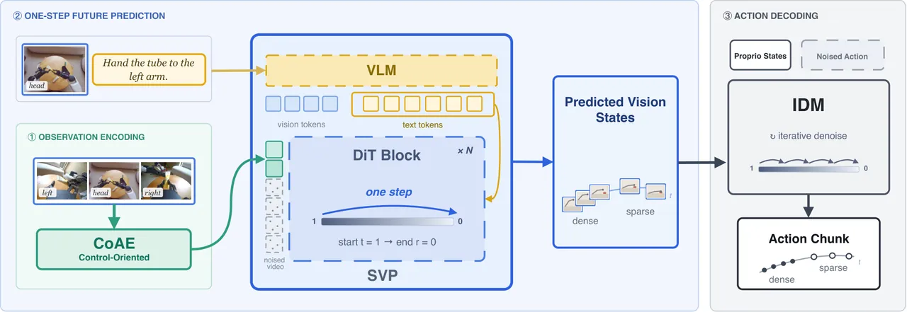
Paper Figure 1: CoAE encodes multi-view observations, SVP predicts the future in one forward pass, and IDM converts current and predicted latents into an action chunk.
4. SVP: a complete future in one generator pass
4.1 Dense near-term and sparse far-horizon prediction
The planner must resolve near-term motion while retaining the task-level intent over a longer horizon. Predicting every control-rate frame across the full clip would spend most tokens far from the immediate action. The paper uses two temporal scales: $$\mathcal{F}=\{f_0\}\cup\left\{f_0+j\frac{H}{N_d}\right\}_{j=1}^{N_d}\cup\left\{f_0+H+\left\lfloor k\frac{T-H}{N_s}\right\rfloor\right\}_{k=1}^{N_s}$$ $f_0$ is the current frame, $N_d$ dense frames span the action-execution horizon $H$, and $N_s$ sparse frames reach the end of the clip $T$. The defaults are $(N_d,N_s,H)=(4,2,52)$ at 30 Hz, so the dense horizon covers about 1.73 seconds.
The IDM receives the complete multi-scale future as context, but the controller executes only the dense action chunk. Sparse actions provide auxiliary supervision over a longer horizon and keep immediate control connected to the task outcome.
4.2 Scene-grounded language through a frozen VLM
An instruction such as "place it behind the red bowl" cannot be grounded by text alone. The referent and relation depend on the current scene. SVP uses a frozen Qwen3.5-2B VLM to jointly encode the head-view image $o_{head}$ and instruction $c$: $$(h_0,h_1,\ldots,h_L)=\mathrm{VLM}(o_{head},c)$$ Only the text-span states are passed to the generator, but those states have already been contextualized by the image.
Different layers contain different mixtures of lexical, spatial, and visual information. A learned gate pools each layer and fuses the text states: $$\alpha_\ell=\mathrm{softmax}_\ell(g(\mathrm{Pool}(h_\ell[\mathcal{T}]))),\qquad c_{vlm}=\mathrm{LN}\left(\sum_{\ell=0}^{L}\alpha_\ell h_\ell[\mathcal{T}]\right)$$ Every diffusion-transformer block cross-attends to $c_{vlm}$. IDM never receives the instruction directly, so language can influence action only through the generated future. This separation is what allows IDM pretraining on instruction-free trajectories.
4.3 Conditional MeanFlow for one-step prediction
For recorded future latents $z$ and Gaussian noise $\epsilon$, the linear path is $z_t=(1-t)z+t\epsilon$ with target velocity $v_c=\epsilon-z$. MeanFlow learns the average velocity over an interval: $$u(z_t,r,t)=\frac{1}{t-r}\int_r^t v(z_\tau,\tau)\,d\tau$$ At $(r,t)=(0,1)$, a single evaluation can map noise to data. A shared DiT trunk predicts the mean velocity $u_\theta$, while an auxiliary head predicts the instantaneous velocity $v_\theta$ and supplies the state tangent.
Observed frames remain clean and only future frames follow the noisy path. Inference then uses one forward pass: $$\hat{z}^{(i)}=z_1^{(i)}-m_i u_\theta^{(i)}(z_1,r=0,t=1)$$ Here $m_i=0$ marks a conditioning frame and $m_i=1$ marks a future frame. The generated latent is differentiable with respect to the generator, so action loss can update both SVP and IDM.
The SVP flow generator has 2.51B parameters. It is a 36-block DiT with width 2048 and 32 attention heads: 20 shared blocks, followed by 8 blocks for the mean-velocity head and 8 parallel blocks for the instantaneous-velocity head. Each view contains one conditioning frame and six predicted frames, or 168 latent tokens.
5. IDM and the validity gap
IDM receives current multi-view latents, predicted futures, and proprioceptive state $s$. It uses cross-attention over the future and produces a dense action chunk plus sparse long-horizon actions. Its action flow-matching loss is: $$\ell_{FM}(a;o,s,z)=\mathbb{E}_{t,\epsilon}\left\|v_\phi(a_t,t;o,s,z)-(\epsilon-a)\right\|^2$$ During separate pretraining, $z$ and $a$ come from the same rollout and are compatible by construction. During co-training, the action still comes from that rollout, but IDM now sees a future $\hat{z}$ produced by SVP.
End-to-end co-training directly backpropagates the action loss through the generated future: $$\hat{z}=G_\theta(o,c,\xi),\qquad \mathcal{L}_{E2E}=\ell_{FM}(a;o,s,\hat{z})$$ This can overwrite the capabilities learned during separate pretraining. Retaining the original video and IDM losses gives: $$\mathcal{L}_{E2E+PT}=\mathcal{L}_{E2E}+\mathcal{L}_{SVP}+\mathcal{L}_{IDM}$$ The added losses reduce forgetting, but they do not fix the mode mismatch between a generated future and the recorded action.
The paper isolates that mismatch in a toy two-stage system. Four Gaussian video modes map to two action modes. When generated futures and recorded actions are paired independently, squared-error regression averages the two conflicting action targets and collapses their bimodal structure. A better generator does not solve the problem because the issue is conditional independence, not visual realism.
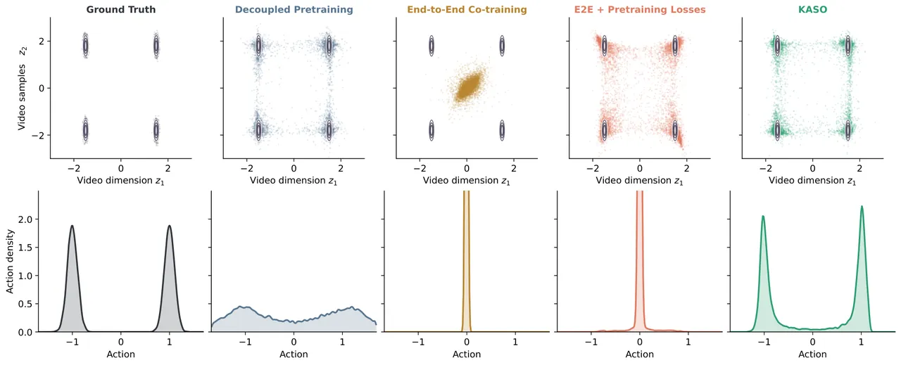
Paper Figure 5: End-to-end training collapses both video and action modes; retaining pretraining losses preserves video modes but not action modes; KASO recovers both.
6. KASO: selecting futures in action space
KASO samples $N$ candidate futures for each context. The active IDM evaluates every candidate and the recorded future under the same high-noise action input. Candidate energy is: $$E_n=\frac{1}{|\mathcal{D}|}\sum_{i\in\mathcal{D}}\left\|v_{\phi,i}(\tilde{a},t_p;o,s,\hat{z}_n)-v_{\phi,i}(\tilde{a},t_p;o,s,z)\right\|_2^2$$ The probe time is $t_p=0.95$. At high noise, the action input carries little information about the target action, so the velocity must be inferred from the visual future. A low energy means the IDM reads similar behavior from the candidate and the recorded future.
KASO selects the top-$k$ candidates, retains their generation noise, and replays the selected futures with gradients. The generated action loss is: $$\mathcal{L}_{E2E}^{sel}=\frac{1}{k}\sum_{n\in\mathcal{S}_k}\ell_{FM}(a;o,s,\hat{z}_n)$$ The complete objective is: $$\mathcal{L}_{KASO}=\mathcal{L}_{E2E}^{sel}+\mathcal{L}_{SVP}+\mathcal{L}_{IDM}$$ The implementation uses $N=4$ and $k=1$. Candidate sampling and scoring run without gradients; replay is differentiable. Selection is recomputed online at every optimizer step, so the compatible candidate set follows the current SVP and IDM.
flowchart LR
  A[Instruction] --> B[Frozen VLM]
  C[Multi-view observation] --> D[CoAE]
  C --> B
  B --> E[Grounded text states]
  D --> F[SVP one-step generator]
  E --> F
  G[Gaussian noise] --> F
  F --> H[Recorded future branch]
  F --> I[Sample N candidate futures]
  H --> J[IDM reference response]
  I --> K[IDM candidate responses]
  J --> L[Action-space energy]
  K --> L
  L --> M[Top-k compatible futures]
  M --> N[Differentiable replay]
  N --> O[Action chunk and joint update]
  H --> P[Recorded-video losses]
  P --> O
KASO changes only the generated-future action branch relative to E2E+PT, so those two methods isolate selection. E2E and E2E+PT isolate the effect of retaining pretraining losses. This controlled decomposition is more informative than comparing only the final policy against unrelated baselines.
7. Data mixture and real-robot scaling
SVP pretraining uses 39,000 hours of instruction-video data, including action-free video. IDM pretraining uses 32,000 hours of action-labeled trajectories, including failures and deployment data. KASO co-training uses 30,000 hours of instruction-video-action data. G1-OP contributes more than half of the co-training mixture; G2-90D contributes less than 2%.
The primary evaluation contains 100 atomic tasks across 20 skill groups. Each task is tested on both G1-OP and G2-90D at 300, 1,200, 5,000, and 30,000 hours, with ten trials per task, embodiment, and scale. Test scenes, backgrounds, lighting, and object instances are excluded from training, and no task-specific fine-tuning is used.
| Co-training data | G1-OP success | G2-90D success | Interpretation |
|---|---|---|---|
| 300 hours | 17.1% | 13.4% | Limited task coverage on both embodiments |
| 1,200 hours | 22.6% | 21.0% | Large gain on the data-scarce embodiment |
| 5,000 hours | 27.3% | 23.5% | Broad but gradual improvement |
| 30,000 hours | 44.1% | 31.1% | Gains of 27.0 and 17.7 points over 300 hours |
Both curves continue to rise between 5,000 and 30,000 hours, so the measured range does not show saturation. Nineteen of twenty G1-OP skill groups and eighteen of twenty G2-90D groups improve from 300 to 30,000 hours. The number of tasks with nonzero success rises from 39 to 76 on G1-OP and from 24 to 72 on G2-90D.
The G2-90D result is important because the embodiment supplies less than 2% of co-training data. Ten of its twenty skill groups receive fewer than five attributed hours; six receive fewer than two hours and four receive fewer than one hour. Flip and Separate reach 20.0% and 16.7% success with only 1.2 and 1.25 hours of G2-specific data. Pass reaches 34.0% with 3.9 hours. These results support cross-embodiment transfer rather than isolated per-robot specialization.
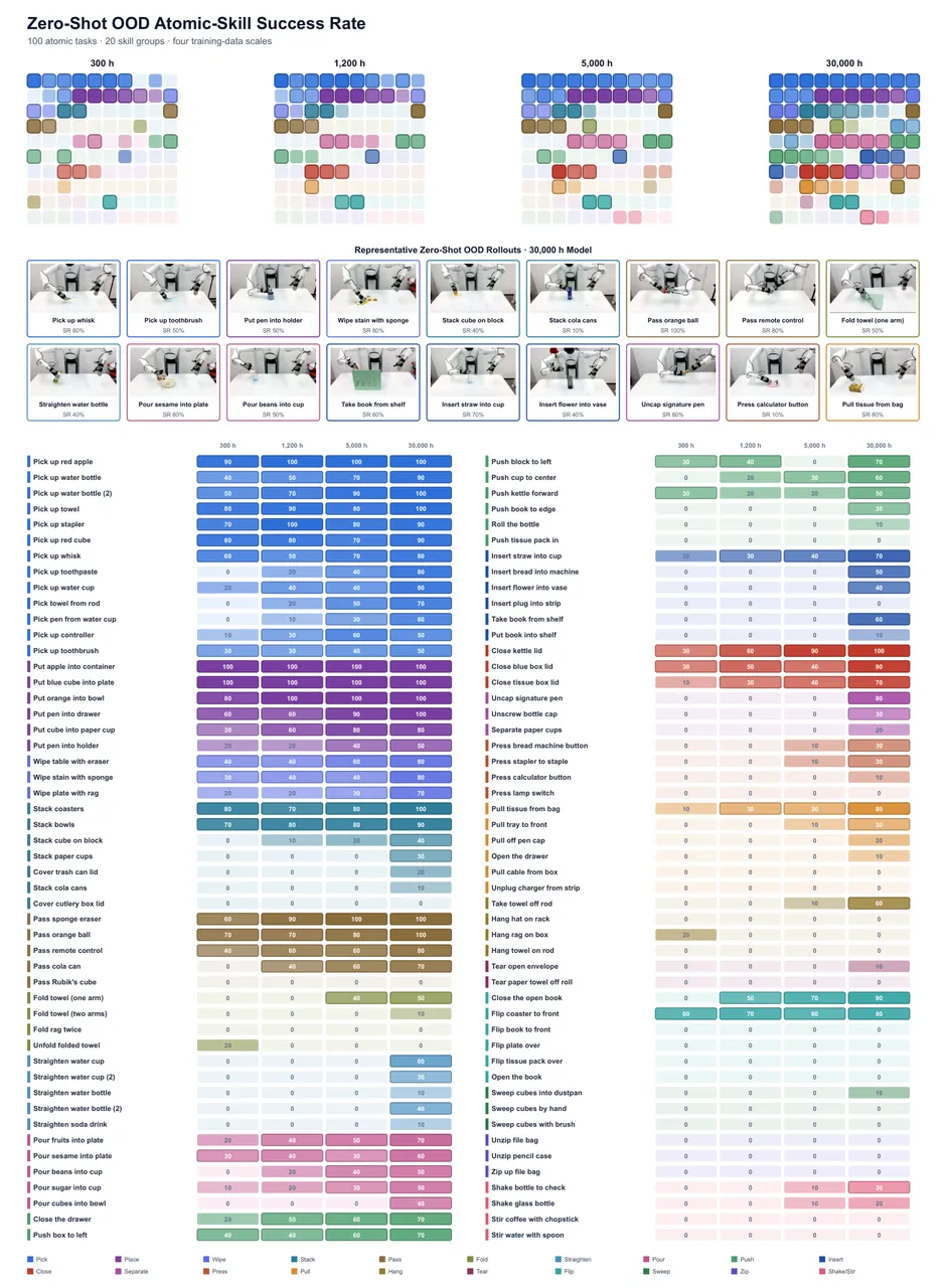
Paper Figure 8: Every G1-OP task is shown across the four co-training scales, with rollouts and per-task success displayed below the task wall.
8. Skill coverage, transfer, and language grounding
The paper maps the full corpus to the same taxonomy as the real-robot suite. After excluding the mechanically simple Close group, skill-specific training hours correlate strongly with G1-OP zero-shot success: Pearson $r=0.80$ and Spearman $\rho=0.85$. The fitted relationship corresponds to 1.94 additional logit units per tenfold increase in coverage.
This relationship explains several otherwise puzzling contrasts. Wipe and Sweep use related surface-contact motions, but Wipe has 824.1 training hours and reaches 76.7% success, while Sweep has 64.6 hours and reaches 3.3%. Stack receives 756.2 hours and reaches 41.4%. Straighten receives 510.5 hours and remains at zero until the largest scale, where it reaches 30.0%.
Instruction grounding is measured on 33 Pick and 26 Place instructions, totaling 295 real-robot trials. The suite separates object, color, size, shape, position, and order. Follow Score is at least 90% for both Pick and Place on object, color, direct position, and shape. It falls to 82.5% and 65.7% for size, and to 13.3% and 26.7% for order.
Overall Follow Score is 83.1%, while full-task success is 72.9%. The gap shows that some failures occur after the policy has reached the correct referent. The training corpus contains size, shape, and order in only 0.96%, 0.67%, and 0.13% of instructions, respectively. That long-tail distribution aligns with the weaker size and order results, although the study establishes association rather than a controlled causal effect.
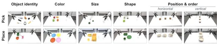
Paper Figure 12: Controlled Pick and Place scenes for object, color, size, shape, position, and order.
Behavioral-conflict tests change the target or commanded arm after the robot has committed to a prior action. The robot briefly retains residual motion toward the old target, then redirects; an arm switch is completed by the new arm with little hesitation. A semantic-conflict test asks the robot to place a cup into a shoebox. The policy follows the explicit relation rather than the more conventional scene association. These are qualitative demonstrations outside the scored evaluation.
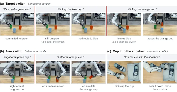
Paper Figure 14: Target switching, arm switching, and counter-conventional semantic conflict.
9. KASO ablation and simulation benchmarks
The controlled real-robot ablation starts every arm from the same full-scale SVP and IDM and uses the same 300-hour alignment mixture. In the four-object scene, KASO and E2E+PT both reach a 95% Follow Score, but KASO raises macro-average pick success from 22.5% to 37.5%. In the single-object scene, pick success rises from 12% to 40%.
| Method | Four-object Follow Score | Four-object pick success | Single-object pick success |
|---|---|---|---|
| E2E | 87.5% | 27.5% | 12% |
| E2E+PT | 95% | 22.5% | 12% |
| KASO | 95% | 37.5% | 40% |
The important change is not target selection but execution after correct contact. KASO preserves the high Follow Score and improves the conversion from contact to completed pick. This is consistent with better behavioral compatibility between generated futures and recorded actions, although the 300-hour alignment setup is deliberately smaller than the final system.
The paper also runs three simulation benchmarks after each benchmark's prescribed in-distribution adaptation. GE-Act 2.0 reaches 76.71%, 70.28%, 65.92%, 66.52%, 70.39%, and 60.52% on RoboTwin's Easy, Background, Light, Clutter, Height, and Hard conditions, respectively, outperforming StarVLA, GR00T-N1.7, and pi-0.5 in every column.
On GenieSim-Instruction, GE-Act 2.0 reaches a normalized average of 0.770, ahead of ACoT-VLA at 0.757, pi-0.5 at 0.746, LingBot-VLA 2.0 at 0.708, and GR00T-N1.7 at 0.646. LIBERO-Plus gives GE-Act 2.0 an overall 80.4%, below pi-0.5 at 84.4%, but it is strongest on camera perturbation at 94.1% and sensor noise at 95.5%, and weaker on robot-state and background shifts.
| Benchmark | GE-Act 2.0 | Strongest comparison | Takeaway |
|---|---|---|---|
| RoboTwin Clean-to-Random | First in all six columns; 60.52% Hard | pi-0.5; 47.90% Hard | Clear advantage under environment and layout shifts |
| GenieSim-Instruction | 0.770 average | ACoT-VLA; 0.757 average | Overall lead, but not first on every task |
| LIBERO-Plus | 80.4% overall | pi-0.5; 84.4% overall | Competitive, with remaining robot/background gaps |
The project page reports 104 ms per action chunk on one RTX 5090, producing 52 executable actions at 30 Hz. One-step future generation and a five-step action-flow sampler keep the full observation-to-action pipeline within real-time control territory.
10. Why the design matters
The main contribution is not a single module but the data and optimization contract between modules. SVP can learn from action-free video, IDM can learn from instruction-free trajectories, and KASO decides which generated futures are suitable for joint action supervision. This makes heterogeneous manipulation data usable without requiring every source to contain the same labels.
CoAE also changes how a control latent should be evaluated. At the same compression factor, DC-AE is worse on both action recovery and instruction matching, while CoAE is competitive with larger-token teachers. Teams building real-time VLA or world models should therefore measure token cost, decodability, and action recoverability together.
KASO requires several conditions to be useful. The generator must produce diverse modes, and the IDM must be sensitive enough to distinguish them at the probe noise level. If every sample is identical, or the IDM cannot extract behavior from the visual future, the energy ranking carries little information. Online selection also adds candidate generation and scoring cost at every optimizer step.
The real-robot result covers two embodiments and establishes transfer to a data-scarce robot, but a 31.1% absolute success rate is not deployment-grade reliability for arbitrary manipulation. The breadth of the 100-task suite is valuable for measuring a repertoire; it does not imply that every difficult contact-rich or deformable task is solved.
11. Limitations
The authors state that egocentric manipulation video has not yet been explored at the scale its availability permits. They view it as a promising source of diverse physical interaction and task semantics, but the paper provides only preliminary signals. The effect of volume, diversity, and mixture composition on downstream capability remains future work.
The authors also position GE-Act 2.0 as a System-1 instruction-conditioned controller. It does not provide explicit deliberation, long-horizon planning, task decomposition, memory, or self-correction. Open-environment execution will require a complementary System-2 layer, and the interaction between such a planner and a scalable world-action model is unresolved.
An independent limitation is that the data-scaling ladder is not a matched-compute experiment. Models train to one epoch or a compute-budget limit, whichever comes first. The 30,000-hour result therefore measures the practical effect of scaling data and optimization together, not an isolated causal effect of data volume alone.
The skill-coverage analysis is also observational. Training hours correlate with difficulty, action complexity, and task composition. Since the study does not independently manipulate skill coverage while holding those factors fixed, the fitted 1.94-logit-per-decade relationship should be treated as an empirical association rather than a precise scaling law.
KASO reduces mismatch by trusting the active IDM as the compatibility judge. If the IDM has a biased estimate for a mode, selection inherits that bias. Future policy optimization may still need additional constraints for action diversity, stability, and safety, especially when generated futures are used in closed-loop training.
12. Conclusion
GE-Act 2.0 provides a complete recipe for from-scratch world-action pretraining: a control-oriented latent space, a one-step visual planner that enables separate SVP and IDM pretraining, and KASO to filter generated futures by action compatibility. Across 100 real-robot tasks, two embodiments, and four data scales, expanding shared manipulation data improves zero-shot out-of-distribution capability, including on an embodiment contributing less than 2% of the training mixture.
The broader lesson is that a world model should be judged not only by the realism of its predictions but by whether those predictions and executable actions occupy the same behavioral mode. KASO turns that interface into a measurable training decision and shifts the evaluation question from visual fidelity toward action compatibility.
The most useful predicted future is not the one that looks most realistic. It is the one that leads to the right action.