PAPER DEEP DIVE
HIL-UMI: Bringing Human-in-the-Loop Post-Training of Vision-Language-Action Models to Universal Manipulation Interface
Large-scale vision-language-action (VLA) models provide powerful priors for robot manipulation, yet adapting them to a specific deployment remains challenging. Supervised fine-tuning (SFT) on task-specific demonstrations provides a step toward deployment, but faces two persistent limitations: static data provide limited coverage of out-of-distribution states, and standard imitation objectives do not distinguish progressing behavior from less useful data. Interactive post-training can address these limitations, but typically requires repeated policy execution and human intervention on a physical robot. We introduce HIL-UMI, a policy-guided Universal Manipulation Interface (UMI) framework for robot-free human-in-the-loop VLA post-training. During handheld UMI demonstrations, HIL-UMI queries the current policy on the same observation stream without executing its predictions. The Energy Score compares the human action trajectory with policy inference and triggers collection when their discrepancy indicates an out-of-distribution region. In a separate feedback loop, low online advantage predictions identify essential segments for refining a progress-based advantage estimator. The updated estimator then guides advantage-conditioned behavioral cloning using a balanced mixture of base demonstrations and new policy data. This design preserves the iterative and policy-aware nature of human-in-the-loop learning while decoupling data collection from robot deployment. Experiments on four real-world tasks spanning long-horizon and precise manipulation show that HIL-UMI achieves consistent improvement over SFT and benefits from both targeted collection and advantage refinement. Moreover, HIL-UMI outperforms HG-DAgger on Clean Up Table with lower per-frame collection time, suggesting a scalable path for VLA post-training across operators and locations.
Paper Metadata
| Item | Content |
|---|---|
| Title | HIL-UMI: Bringing Human-in-the-Loop Post-Training of Vision-Language-Action Models to Universal Manipulation Interface |
| Authors | Zimu Han, Yiming Zeng, Jiyao Zhang, Zihao Zhao, Yuanfei Wang, Yixiang Jin, Shiqi Li, Shuangben Chen, Wei Huang, Ruodai Li, Hui Shen, Hao Dong (corresponding) |
| Affiliations | Peking University, Xi'an Jiaotong University, JD Technology, PrimeBot |
| Submitted | 2026-09-17, arXiv:2609.20659 (cs.RO) |
| Links | arXiv abstract · arXiv full text · project page |
| Code status | Not released. The project page is a JS-rendered landing page with no repository link; GitHub searches by title and authors return no implementation repo, so this paper provides no public code |
| Hardware | Collection: custom handheld UMI device (AgiBot OmniPicker gripper + Meta Quest 3 controller/headset + RealSense D405 wrist camera + D455 third-person camera). Evaluation: single Franka Panda arm. Online inference: one RTX 4090D |
One-Sentence Summary
HIL-UMI moves human-in-the-loop VLA post-training off the robot: while an operator demonstrates with a handheld UMI gripper, the current policy runs $N=10$ stochastic inferences on the same observation stream without executing its predictions, an Energy Score measures the discrepancy between the human action chunk and the policy's action-chunk distribution to flag out-of-distribution (OOD) states for targeted collection, a second loop harvests segments where the advantage estimator under-predicts progress to retrain itself, and advantage-conditioned behavioral cloning (ACBC) then consumes a balanced mix of old and new data. On four real tasks it beats SFT throughout (Stack Cube 84 to 100 TPS in three rounds) and collects 5.63x faster per frame than real-robot HG-DAgger (73.40 vs 412.99 ms/frame).
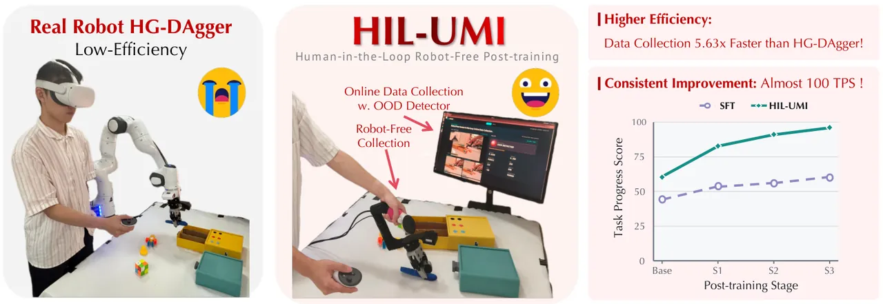
Fig. 1: Paper teaser. Left: real-robot HG-DAgger needs policy rollouts and human takeovers on the arm. Middle: HIL-UMI collects robot-free with an online OOD detector. Right: headline results, 5.63x faster collection and near-100 TPS on Clean Up Table.
Background and Motivation
Large-scale vision-language-action (VLA) models acquire broad manipulation priors from diverse robot and vision-language data, and they are strong initializations for downstream robot learning. Broad competence, however, does not translate into reliable execution in a specific deployment: the target embodiment, observation setup, workspace, dynamics, and required precision can all differ from pretraining. Task-specific post-training is therefore the bridge between general representations and robust closed-loop behavior, and it matters most for long-horizon and precise manipulation, where small local errors decide whole-task success.
The dominant adaptation recipe collects task demonstrations on physical robots and applies supervised fine-tuning (SFT). Two core problems survive this recipe. First, behavioral cloning suffers from covariate shift and compounding errors: static demonstrations cover mostly expert-visited states, so once the policy makes a small mistake it slides into regions the data never saw, and more nominal demonstrations do not repair those policy-induced OOD states. Second, standard imitation objectives weight every demonstration sample equally, with no notion of which segments actually advance the task and which are redundant nominal motion.
Human-in-the-loop post-training attacks both problems at once. DAgger queries expert actions at learner-visited states and aggregates them into the training set, directly expanding coverage of policy-induced states; human-gated and real-robot variants add teleoperation, rollouts, interventions, or reward feedback around policy failures; RECAP folds demonstrations, autonomous on-robot experience, and teleoperated corrections into advantage-conditioned policy training. The catch is that the corrective signal ultimately lives on a physical robot: repeated deployment is expensive, hard to parallelize across operators and locations, and teleoperation makes long-horizon, high-precision demonstrations difficult to collect at scale.
The Universal Manipulation Interface (UMI) offers an escape from the robot: portable handheld grippers record robot-compatible observations and actions, direct hand demonstrations express complex and precise behaviors naturally, and portability allows collection across operators and locations. Follow-ups such as FastUMI, MV-UMI, and HiFi-UMI improve the hardware stack, add third-person views, and raise trajectory fidelity, with HiFi-UMI showing UMI-only post-training can approach real-robot teleoperation. Yet their real-time feedback targets sensing and capture quality, not the current policy's predictions, so collection stays centered on data fidelity and general coverage rather than the policy's specific blind spots.
HIL-UMI fills exactly that gap: it keeps the iterative, policy-aware nature of human-in-the-loop learning while decoupling data collection from robot deployment. As the human demonstrates with the handheld device, the current policy predicts actions from the same observation stream without executing them, and the discrepancy between prediction and demonstration decides whether the state is OOD and worth extra data. The paper contributes (i) a UMI-based human-in-the-loop framework that moves iterative VLA post-training off the robot, (ii) a real-time OOD detector that compares human action trajectories against the policy's trajectory distribution plus an iterative workflow that updates an advantage model and runs ACBC every round, and (iii) validation on four long-horizon or precise real tasks with consistent gains over SFT and better performance plus higher collection efficiency than HG-DAgger.
Preliminaries
The UMI data format underpins everything. The operator records synchronized observations $o_t$ (wrist plus third-person camera) and human action chunks $H_t=(h_{t,1},\ldots,h_{t,T})$ at 30 Hz; a demonstration $\tau_i=\{(o_{i,t},a_{i,t})\}_{t=0}^{L_i-1}$ is an observation-action sequence. Each action $a_k=(p_k,R_k,g_k)$ holds end-effector position, orientation, and gripper command, matching the Franka evaluation arm's action space so UMI data trains robot policies directly.
The second prerequisite is policy sampleability. The base policy is the open-source $\pi_{0.5}$, a flow-based VLA: given an observation and instruction it can draw multiple stochastic action chunks rather than emit a single deterministic action or a Gaussian. The policy's action distribution can therefore be approximated empirically, but no analytic likelihood exists, which motivates the Energy Score rather than a likelihood-ratio test for OOD detection.
The third prerequisite is advantage-conditioned behavioral cloning (ACBC) with a two-observation advantage estimator. The RECAP line of work shows that writing data quality into the conditioning (a positive or negative advantage label appended to the prompt) lets a policy exploit suboptimal data in training while favoring high-advantage behavior at inference. HIL-UMI keeps that idea but sources the advantage from a regressor $f_\psi(o_u,o_v,c)$ that predicts relative task progress from $o_u$ to $o_v$ directly, avoiding the compounding error of differencing two independent predictions.
Method
The round loop and base initialization
Let $c$ be the task instruction and $\mathcal{D}_0=\{\tau_i\}_{i=1}^M$ the initial UMI dataset. Post-training runs rounds $r=1,\ldots,R$, and each round collects two separate datasets with equal frame budgets, $|\mathcal{D}_r^A|=|\mathcal{D}_r^P|$: $\mathcal{D}_r^A$ refines the advantage estimator and $\mathcal{D}_r^P$ improves the policy. Before round 1, base initialization assigns progress targets to $\mathcal{D}_0$, trains $f_{\psi_0}$, labels the same demonstrations with binary advantage labels, and obtains the base policy by ACBC,
$$\theta_0=\arg\min_\theta\ \mathbb{E}_{(o,a,b)\sim\mathcal{D}_0}\left[\ell_{\mathrm{BC}}\bigl(\pi_\theta(\cdot\mid o,c^b),a\bigr)\right], \qquad (1)$$
where $\ell_{\mathrm{BC}}$ is the policy's native action-prediction loss, $b$ the advantage label, and $c^b$ the label-augmented prompt. Note that this step already uses only advantage-conditioned cloning on the base data, which is why HIL-UMI's Base point in Fig. 5 sits above SFT's. Within each round the order is: run $f_{\psi_{r-1}}$ online to collect $\mathcal{D}_r^A$; run $\pi_{\theta_{r-1}}$ alongside the human UMI demonstration and collect $\mathcal{D}_r^P$ where the policy's action distribution is flagged OOD; continue training from $\psi_{r-1}$ on a balanced mixture to get $\psi_r$; finally label data with $f_{\psi_r}$ and continue ACBC from $\theta_{r-1}$ to get $\theta_r$.
Policy OOD collection: Energy Score between human and policy
The paper operationalizes OOD as task situations poorly represented in a model's training data, flagged by inconsistencies between model predictions and human demonstrations. At observation $o_t$ the operator produces a human action chunk $H_t$ while the system performs $N=10$ stochastic policy inferences at the same observation and instruction,
$$A_t^{(n)}\sim\pi_{\theta_{r-1}}(\cdot\mid o_t,c),\qquad n=1,\ldots,N, \qquad (2)$$
an empirical approximation of the policy's action-chunk distribution. Sampling runs concurrently with UMI collection, but comparison happens only after the human chunk is complete. Writing the $k$-th action as $a_k=(p_k,R_k,g_k)$, chunks $A$ and $B$ are compared in a common coordinate frame by
$$\rho^2(A,B)=\frac{1}{T}\sum_{k=1}^T\left[\lambda_p\lVert p_k^A-p_k^B\rVert_2^2+\lambda_R\,d_R(R_k^A,R_k^B)^2+\lambda_g\lVert g_k^A-g_k^B\rVert_2^2\right], \qquad (3)$$
with orientation differences measured by the geodesic distance on $\mathrm{SO}(3)$,
$$d_R(R_1,R_2)=\arccos\!\left(\frac{\operatorname{tr}(R_1^\top R_2)-1}{2}\right). \qquad (4)$$
The coefficients are $(\lambda_p,\lambda_R,\lambda_g)=(0.5,0.25,0.25)$. The discrepancy between the single human chunk and the predicted distribution is then the empirical Energy Score,
$$\operatorname{ES}(H_t)=\frac{1}{N}\sum_{n=1}^N\rho\bigl(A_t^{(n)},H_t\bigr)-\frac{1}{2N(N-1)}\sum_{n\neq m}\rho\bigl(A_t^{(n)},A_t^{(m)}\bigr). \qquad (5)$$
The first term measures how far policy samples lie from the human action; the second subtracts the dispersion of the policy samples so the criterion does not collapse to an average pointwise error. The balance makes the score sensitive to both location and predictive spread: excessive spread raises sample-to-human distances, while a collapsed distribution far from the human action receives no diversity correction. The score needs neither a Gaussian assumption nor an explicit likelihood, which suits flow-based policies. A large Energy Score means the demonstrated solution lies outside the policy's predictive distribution, and the state region is treated as OOD. The detector is therefore
$$\delta_t^P=\mathbb{I}\!\left[\operatorname{ES}(H_t)>\tau_P\right], \qquad (6)$$
with a threshold $\tau_P$ shared across all tasks. When a completed chunk triggers $\delta_t^P=1$, the operator records an expert demonstration from the current state until the current subtask is completed; repeating this yields $\mathcal{D}_r^P$, concentrating the policy update on states where the current action distribution does not cover the human solution, all without executing the policy.
Advantage OOD collection: harvesting under-predicted progress
The second collection stream targets the advantage estimator itself. In round $r$, whenever $t\geq K$, relative task progress is estimated from an observation pair with a $K$-frame offset,
$$\widehat{A}_t^{\mathrm{online}}=f_{\psi_{r-1}}(o_{t-K},o_t,c),\qquad \delta_t^A=\mathbb{I}\!\left[\widehat{A}_t^{\mathrm{online}}<\tau_A\right]. \qquad (7)$$
The threshold $\tau_A$ is calibrated per task with the initial estimator $f_{\psi_0}$: evaluate $f_{\psi_0}$ on base-data observation pairs separated by $K$ frames, take the empirical cutoff $\kappa_0$ that selects the top $\eta$ fraction of predicted advantages ($\eta=0.3$, the same cutoff used for base-data labeling), and set $\tau_A=\kappa_0/2$, adapting to each task's progress scale over the fixed temporal interval. The semantics are clean: assuming the operator demonstrates task-progressing behavior, predictions below the calibrated threshold mark segments where the estimator may underestimate progress, i.e. hard cases for the advantage model. On a trigger, the operator records from the current state through the end of the subtask, forming $\mathcal{D}_r^A$.
Advantage model: linear progress targets and segmental regression
Rather than differencing two independently predicted values, $f_\psi(o_u,o_v,c)$ regresses relative task progress from $o_u$ to $o_v$ directly, reducing compounding estimation error. To accommodate both full base episodes and the intentionally truncated segments collected in later rounds, progress targets are linear. For base episodes,
$$z_{i,t}=\frac{t}{L_i-1},\qquad t=0,\ldots,L_i-1, \qquad (8)$$
with average base-episode length $\overline{L}_0=\frac{1}{M}\sum_{i=1}^M L_i$ (Eq. 9). An iterative segment $\sigma_{r,j}$ of length $L_{r,j}$ ends when its subtask is completed; assigning it the full $[0,1]$ range would overstate its progress, so instead
$$z_{r,j,t}=\frac{t}{L_{r,j}-1}\cdot\frac{L_{r,j}}{\overline{L}_0},\qquad t=0,\ldots,L_{r,j}-1, \qquad (10)$$
which spans $0$ to $L_{r,j}/\overline{L}_0$ and keeps the temporal progress scale consistent with the base data. Training uniformly samples two distinct frames $u,v$ from the same trajectory or segment with signed target $y_{u,v}=z_v-z_u$ and optimizes, over multiple temporal spans,
$$\mathcal{L}_A(\psi)=\mathbb{E}_{(o_u,o_v,y_{u,v})}\left[\bigl(f_\psi(o_u,o_v,c)-y_{u,v}\bigr)^2\right]. \qquad (11)$$
Mixing and the two model updates
To balance current-round hard cases against history, the paper defines a mix operator
$$\operatorname{Mix}(\mathcal{D}_{\mathrm{new}},\mathcal{D}_{\mathrm{hist}})\triangleq\alpha\cdot\operatorname{Unif}(\mathcal{D}_{\mathrm{new}})+(1-\alpha)\cdot\operatorname{Unif}(\mathcal{D}_{\mathrm{hist}}), \qquad (12)$$
with uniform sampling and $\alpha=0.5$. The advantage training set is $\widetilde{\mathcal{D}}_r^A=\operatorname{Mix}\bigl(\mathcal{D}_r^A,\bigcup_{j<r}\mathcal{D}_j^A\bigr)$ (Eq. 13); continuing from $\psi_{r-1}$ and minimizing Eq. (11) yields $\psi_r$. The policy training set is symmetric, $\widetilde{\mathcal{D}}_r^P=\operatorname{Mix}\bigl(\mathcal{D}_r^P,\bigcup_{j<r}\mathcal{D}_j^P\bigr)$ (Eq. 14). The updated estimator then scores every eligible base sample over the same future horizon,
$$\widehat{A}_{r,t}=f_{\psi_r}(o_t,o_{t+K},c),\qquad t+K<L, \qquad (15)$$
and binary labels follow the top-$\eta$ cutoff $\kappa_r$ of base-data predictions:
$$b_{r,t}=\begin{cases}\mathbb{I}[\widehat{A}_{r,t}\geq\kappa_r], & (o_t,a_t)\in\mathcal{D}_0,\\[4pt] 1, & (o_t,a_t)\in\bigcup_{j=1}^{r}\mathcal{D}_j^P.\end{cases} \qquad (16)$$
Base samples keep the thresholding rule in every round, while all newly collected policy samples receive positive labels, since they are corrective data gathered around the policy's blind spots. The round-$r$ policy objective is
$$\mathcal{L}_{\mathrm{ACBC}}(\theta)=\mathbb{E}_{(o,a,b)\sim\widetilde{\mathcal{D}}_r^P}\left[\ell_{\mathrm{BC}}\bigl(\pi_\theta(\cdot\mid o,c^b),a\bigr)\right]. \qquad (17)$$
Training continues from $\theta_{r-1}$ and inference uses the positive-advantage prompt to favor task-progressing behavior; $\theta_r$ and $\psi_r$ then enter the next collection round. Engineering-wise, both detectors run in real time on a single RTX 4090D: the policy OOD detector parallelizes the $N$ stochastic samples for 112 ms latency, and the advantage OOD detector takes 93 ms, fast enough to sit inside the human collection loop.
flowchart TD
  subgraph S0["Initialization r=0"]
    D0["Base UMI demos D0
linear progress targets Eq 8"] --> F0["Train advantage estimator f_psi0
regression Eq 11"]
    F0 --> B0["Top eta=0.3 of base predictions
binary labels Eq 16"]
    B0 --> T0["ACBC base policy theta0
Eq 1"]
  end
  subgraph S1["Round r online collection Sec III-A"]
    AC["Advantage loop: f_psi r-1 scores o_t-K vs o_t
below tau_A means underestimated progress, record Eq 7"]
    PC["Policy loop: N=10 stochastic inferences Eq 2
Energy Score above tau_P flags OOD, record Eq 5 Eq 6"]
  end
  subgraph S2["Round r model updates"]
    AU["Mix new and old, continue training
Eq 12 Eq 13 gives psi_r"]
    PU["Relabel with f_psi_r, ACBC on mixed data
Eq 14 to Eq 17 gives theta_r"]
  end
  T0 --> AC
  AC --> PC
  PC --> AU
  AU --> PU
  PU --> NX["theta_r and psi_r enter round r+1"]
  NX --> AC
Redrawn from the paper's Fig. 2: each round runs advantage OOD collection, then policy OOD collection, then updates the advantage estimator and the policy in sequence.
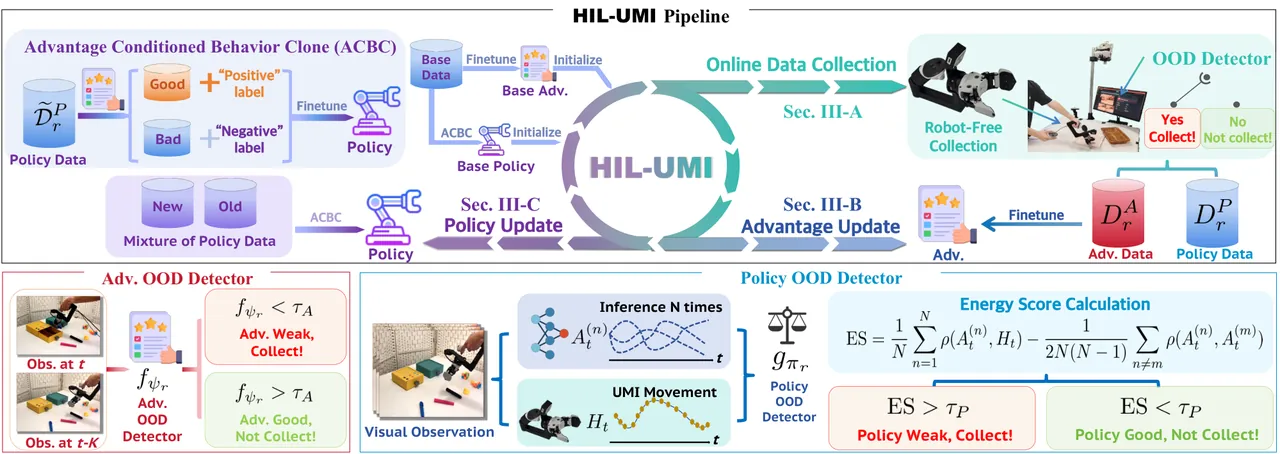
Fig. 2: Original overview. The upper ring is the round loop (online collection, advantage update, policy update); the lower panels unpack the two detectors: the advantage detector compares predicted progress between $o_{t-K}$ and $o_t$ against $\tau_A$, and the policy detector computes the Energy Score between $N$ inferences and the human chunk $H_t$ against $\tau_P$.
Experiments
Tasks, hardware, and protocol
The collection device (Fig. 3) couples an AgiBot OmniPicker gripper to a Meta Quest 3 controller through a custom connector; the Quest 3 headset-controller tracking measures device pose in real time, providing the human action trajectories needed for online OOD detection. A RealSense D405 on the device captures wrist views and a fixed RealSense D455 provides the third-person view, at 30 Hz. Evaluation uses a single Franka arm on four tasks (Fig. 4): Fold Towel (flatten a randomly initialized towel, fold twice while removing wrinkles, place in a basket), Clean Up Table (open the yellow drawer, sort three pens into color-matched slots, close it, then open the blue drawer, put away three toys, close it), Stack Cube (grasp a purple cube and place it on a red cube), and Stamp (grasp a stamp and align it inside a marked box whose length and width exceed the stamp body by only 1 cm).
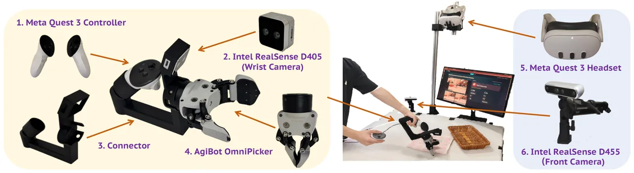
Fig. 3: Hardware. Left: Quest 3 controller, RealSense D405, custom connector, and AgiBot OmniPicker gripper assembly. Right: collection scene with the Quest 3 headset and the RealSense D455 third-person camera.
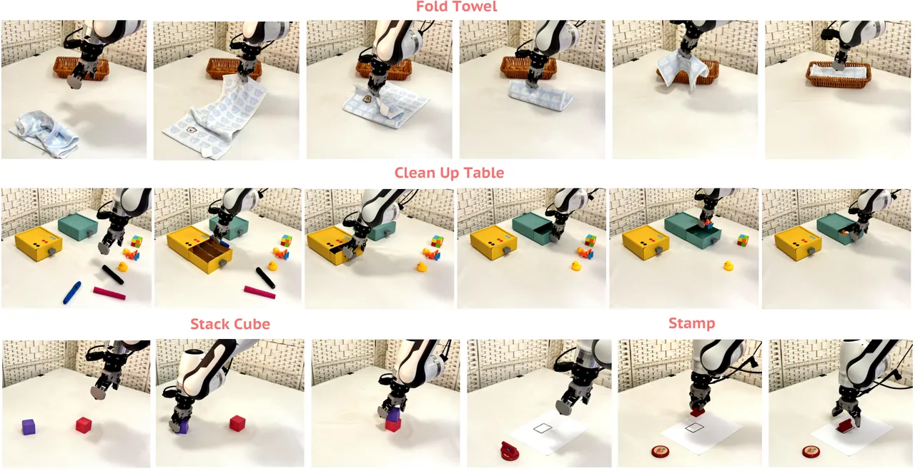
Fig. 4: Execution sequences of the four real-world tasks on the Franka Panda: Fold Towel, Clean Up Table, Stack Cube, Stamp.
Each checkpoint is evaluated for 10 trials per task, with initial object placement varied inside a 30 cm x 60 cm workspace to probe spatial generalization. The metric is Task Progress Score (TPS), partial credit over predefined subtasks on a 0-100 scale; Table 1 lists the scoring criteria (e.g. Fold Towel grants +25 per subtask and deducts 5 points per subtask if the towel is wrinkled or misaligned; Stack Cube deducts 15 points for grasping only one corner).
| Task | Subtasks | Score |
|---|---|---|
| Fold Towel | Flatten / first fold / second fold / place in basket | +25 each |
| Clean Up Table | Pen in matched slot x3 / toy put away x3 / open drawer x2 / close drawer x2 | +10 each |
| Stack Cube | Grasp purple cube / move near red cube / place on red cube | +30 / +30 / +40 |
| Stamp | Grasp stamp / move near box / orient correctly / contact paper / body inside box | +20 each |
Table 1: TPS scoring criteria (paper Table I).
Training configuration and budgets
The base policy is the open-source $\pi_{0.5}$. Long-horizon tasks (Fold Towel, Clean Up Table) use 50 base demonstrations and a 12,000-frame per-round budget; precise tasks (Stack Cube, Stamp) use 80 base demonstrations and 2,500 frames per round. The SFT baseline collects conventional UMI demonstrations under the same budgets. Shared settings (Table 2): 224x224 inputs, action horizon 20, AdamW, policy LR 1e-5, advantage LR 5e-5, cosine schedule with 500 warmup steps, batch 128, weight decay 1e-10, 5000 update steps per round; on the collection side $N=10$, $(\lambda_p,\lambda_R,\lambda_g)=(0.5,0.25,0.25)$, $K=50$, $\alpha=0.5$, $\eta=0.3$.
| Hyperparameter | Value |
|---|---|
| Input resolution / action horizon | 224x224 / 20 |
| Optimizer / schedule | AdamW / cosine, 500 warmup steps |
| Policy / advantage learning rate | 1e-5 / 5e-5 |
| Batch / weight decay / steps per round | 128 / 1e-10 / 5000 |
| Stochastic samples N / Energy Score weights | 10 / (0.5, 0.25, 0.25) |
| Advantage interval K / mix ratio alpha / positive fraction eta | 50 / 0.5 / 0.3 |
Table 2: Implementation hyperparameters (paper Table II).
Main results: consistent separation under equal budgets
Fig. 5 compares SFT, HIL-UMI without the advantage module (w/o Adv., ACBC replaced by plain finetuning on the mixed dataset), and full HIL-UMI under the same per-round budget. Three readings stand out. First, the starting points already differ: HIL-UMI's Base (the ACBC base policy of Eq. 1) sits above SFT's Base on most tasks, e.g. 84 versus about 48 on Stack Cube (matching the Base column of Table 3) and about 75 versus about 56 on Stamp, so merely re-reading the same base data through advantage labels already pays. Second, across rounds SFT improves only marginally and even regresses temporarily (its Clean Up Table curve dips between Iter2 and Iter3), while HIL-UMI climbs monotonically on all four tasks, reaching 100 on Stack Cube and Stamp after three rounds and about 95 on the four-task average against roughly 59 for SFT. Third, removing advantage conditioning costs real performance (Stack Cube 90 versus 100 at round 3, average about 88 versus about 95), because the update then treats task-progressing and suboptimal examples alike. The paper's reading is that extra nominal demonstrations do not cover the states the current policy visits, whereas concentrating the same budget on policy-specific OOD regions and digesting it through advantage-conditioned updates does.

Fig. 5: TPS versus post-training round (Base, Iter1-3) on the four tasks plus the four-task average, for SFT, HIL-UMI w/o Adv., and HIL-UMI (paper Fig. 5).
Threshold ablation: moderate triggers win
Table 3 varies one online trigger at a time on Stack Cube with the other fixed at the selected setting $(\tau_P,\tau_A)=(1.2,0.2)$. The pattern is consistently middle-is-best: a too-permissive $\tau_P$ (0.5) collects low-information states where the policy already agrees with the human and ends at 90 after three rounds; a too-conservative $\tau_P$ (2.0) misses useful policy failures and ends at 96; a loose $\tau_A$ (0.3) injects redundant refinement data (96) while a tight one (0.1) misses informative estimator errors (92). HIL-UMI beats SFT under every tested setting, so the gains do not hinge on a narrowly tuned threshold but on balancing coverage against selectivity.
| (tau_P, tau_A) | Base | Round 1 | Round 2 | Round 3 |
|---|---|---|---|---|
| (1.2, 0.2) | 84 | 86 | 90 | 100 |
| (2.0, 0.2) | 84 | 76 | 86 | 96 |
| (0.5, 0.2) | 84 | 80 | 72 | 90 |
| (1.2, 0.3) | 84 | 76 | 82 | 96 |
| (1.2, 0.1) | 84 | 82 | 82 | 92 |
Table 3: Online collection threshold ablation on Stack Cube, TPS (paper Table III).
Collection efficiency: costlier per frame, but every frame counts
Table 4 shows HIL-UMI costs more milliseconds per recorded frame than SFT on all four tasks (Fold Towel 91.92 vs 69.43, Clean Up Table 73.40 vs 41.70, Stack Cube 89.89 vs 77.04, Stamp 101.02 vs 64.30), because online selection waits for triggered subtask segments. Fig. 6(a) plots four-task mean TPS against cumulative collection time and reverses the verdict: HIL-UMI's mean TPS rises steadily while SFT plateaus and temporarily regresses, so the selection overhead is offset by collecting around policy-specific blind spots with task-progressing supervision. The comparison with real-robot HG-DAgger on Clean Up Table under the same per-stage budget (Fig. 6(b)) is sharper: HIL-UMI leads at every stage and finishes about five TPS points higher, while HG-DAgger needs 412.99 ms per frame, 5.63x the 73.40 ms per frame of HIL-UMI. Avoiding robot rollouts is where that efficiency comes from.
| Task | SFT (ms/frame) | HIL-UMI (ms/frame) |
|---|---|---|
| Fold Towel | 69.43 | 91.92 |
| Clean Up Table | 41.70 | 73.40 |
| Stack Cube | 77.04 | 89.89 |
| Stamp | 64.30 | 101.02 |
Table 4: Collection efficiency comparison (paper Table IV).
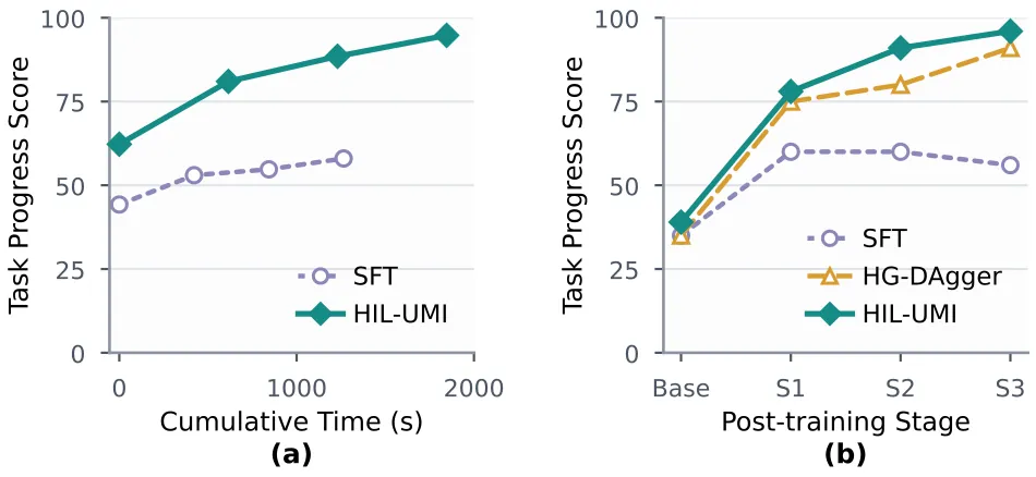
Fig. 6: (a) Four-task mean TPS against cumulative collection time for SFT and HIL-UMI. (b) TPS per stage (Base, S1-S3) on Clean Up Table for SFT, HG-DAgger, and HIL-UMI (paper Fig. 6).
Limitations
First, the authors state the scaling boundary themselves: the current framework is a single operator at a single location, and they position a distributed post-training system with concurrent collection across locations as future work. The 5.63x per-frame advantage demonstrates that parallelization is possible in principle, but merging multi-operator data and calibrating thresholds across people remain unvalidated.
Second, the per-frame collection cost is a designed-in price: Table 4 shows HIL-UMI above SFT on every task, up to 101.02 vs 64.30 ms/frame. The paper offsets this with the TPS-versus-time curves of Fig. 6(a), yet that argument rests on a four-task mean over three rounds; tasks whose OOD triggers are extremely sparse or extremely dense could change the time-efficiency picture, and no ablation covers that regime.
Third, the experimental surface is narrow: one Franka arm, four tasks, and a single base policy ($\pi_{0.5}$). The embodiment gap between human hand motion and robot end-effector actions (gripper speed, force control, kinematic limits) is not modeled explicitly; the OOD criterion simply assumes both live in a comparable action space. Cross-embodiment and cross-backbone generalization stay open.
Fourth, calibration retains manual knobs: $\tau_P$ is shared across tasks but chosen empirically (the ablation covers one task only), and $\tau_A$ needs per-task calibration of $\kappa_0$ on base data. The advantage estimator also leans on visually discernible progress; subtasks whose progress is occluded or ambiguous from two frames (for example operations inside a drawer) give the regressor an unreliable target. Finally, 10 trials per checkpoint per task with a partial-credit TPS metric should not be read as success-rate evidence.
Conclusion and Outlook
HIL-UMI's central move is a relocation: the interaction that human-in-the-loop post-training usually performs on robot rollouts is moved onto the handheld UMI observation stream, where disagreement between policy predictions and human demonstrations replaces policy execution and human takeovers. The Energy Score gives flow-based policies a likelihood-free, distribution-level OOD criterion; the dual collection loops price the policy's blind spots and the advantage model's blind spots separately; ACBC with the Mix operator keeps new and old data from drowning each other during updates. Consistent gains over SFT on four tasks, plus 5.63x collection efficiency over HG-DAgger, support the claim that post-training can scale the way data collection scales.
The next steps are visible from the paper itself: concurrent multi-operator collection with consistent data merging and threshold calibration, explicit modeling of the UMI-to-robot embodiment gap, and advantage estimators robust to visually ambiguous progress. If the code and collection protocol ship with the camera-ready version, HIL-UMI's policy-guided collection interface could become a standard component of the UMI ecosystem, next to fidelity-oriented work like HiFi-UMI.
Golden Quote
"This design preserves the iterative and policy-aware nature of human-in-the-loop learning while decoupling data collection from robot deployment."
(From the paper abstract.)