IMLE-VLA: Fast Single-Step Action Generation for Vision-Language-Action Policies

Paper Metadata

Field	Detail
Title	IMLE-VLA: Fast Single-Step Action Generation for Vision-Language-Action Policies
Authors	Kian Hosseinkhani, Qinhe Peng, George Shramko, Mehran Aghabozorgi, Jianing Qian, Tristan Engst, Alireza Moazeni, Dinesh Jayaraman, Ke Li (corresponding author)
Affiliations	Simon Fraser University; University of Pennsylvania; Alberta Machine Intelligence Institute (Amii), Canada CIFAR AI Chair
arXiv	2609.10915v1 (2026-09-10, cs.RO), submitted to IROS 2026
Project page	kianhk6.github.io/IMLE-VLA. The abstract states "Videos and code are available" at this page, but as of writing it hosts demo videos only, with no runnable training or inference code released.
Model	Frozen $\pi_{0.5}$ 3B vision-language backbone (parameters untouched) plus a single-step conditional generator $G_\theta$ as the action head. $G_\theta$ is initialized from the pretrained $\pi_{0.5}$ checkpoint and is the only component fine-tuned.
Objective	Conditional Implicit Maximum Likelihood Estimation (cIMLE, Li et al. 2018) with sample factor $m = 2$, replacing the 10-step Euler conditional flow matching (CFM) head.
Evaluation hardware	Simulation: one NVIDIA L40S; the frequency benchmark includes the mandatory per-call cost of tokenizing the language instruction and proprioceptive state, averaged over 50 episodes on 10 LIBERO-Long tasks. Real robot: Franka Emika Panda with an NVIDIA A6000, wrist and scene cameras, policies trained on DROID and deployed zero-shot, 20 episodes per task.
Headline numbers	Inference frequency 55 Hz ($3.67\times$); action throughput 1,650 Hz at $H{=}30$ ($11.0\times$); 98.0% average success over the 40-task LIBERO benchmark, the highest among all compared methods; on the real robot VLA-only wall-clock drops $3.9\times$-$6.6\times$ and proprioceptive jerk drops $2.2\times$-$3.0\times$.

One-Sentence Summary

IMLE-VLA removes the iterative action head from $\pi_{0.5}$ entirely: instead of integrating a learned velocity field over 10 Euler steps, a single-step generator trained with a winner-takes-all nearest-neighbour objective (cIMLE) emits a whole action chunk in one forward pass, lifting inference from 15 Hz to 55 Hz ($3.67\times$), compounding to $11.0\times$ action throughput with a longer execution horizon, while scoring the best LIBERO average (98.0%), holding $\pi_{0.5}$'s robustness under LIBERO-plus perturbations, and beating $\pi_{0.5}$ on all four real-robot tasks with $2.2\times$-$3.0\times$ lower jerk.

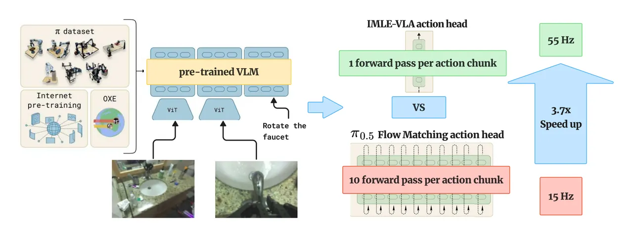
Figure 1 (paper Fig. 1): overview of IMLE-VLA. A single-step action head is dropped into an existing VLA, removing the iterative modelling loop from action generation while the VLM backbone stays unchanged.

Background and Motivation

Vision-language-action (VLA) policies are the dominant generalist paradigm in robot learning because they inherit internet-scale visual and linguistic knowledge from pretrained vision-language models, which buys strong generalization across tasks and embodiments. The authors open by naming the price of that generalization: it is expensive. A large vision-language backbone combined with an iterative action-sampling procedure makes VLA inference a critical bottleneck for high-frequency real-time control. Under synchronous execution the latency becomes dead time in the control loop, because the robot stalls until the next prediction is ready. The visible consequence is stop-and-go execution and longer task completion times.

The paper attributes the bottleneck to the way VLAs generate actions, and identifies two dominant paradigms. The first is autoregressive decoding of discrete tokens, where each action is represented as a token sequence and decoded one token at a time (RT-2, OpenVLA and successors). Beyond the latency of serial decoding, discrete tokenization can limit the fine-grained continuous precision that dexterous manipulation needs. The second generates continuous actions by multi-step sampling with diffusion or flow matching, typically through an action expert attached to a VLM backbone, which is the $\pi_{0.5}$ design. These models predict a chunk of future actions jointly, but producing one chunk still costs multiple sequential forward passes, 10 Euler steps in $\pi_{0.5}$. Action generation therefore remains the primary obstacle to real-time control.

The reason diffusion and flow-matching heads are used at all is their capacity to handle the inherent multimodality of robot action distributions. One instruction such as "clear the table" admits many valid action sequences, and these models are designed to represent that structure. The obvious shortcut, replacing iterative generation with a single-step regression head, has a well-characterized failure mode: the regression objective averages over valid modes and pulls the prediction toward a single mean behaviour, which degrades performance whenever the action distribution is multimodal. The authors validate this empirically in Sec. IV-C through the $m{=}1$ ablation.

That tension frames the central question of the paper: can a single-step generator with a mode-covering objective replace iterative action generation while also improving task performance? The wording matters. The target is not a favourable speed-accuracy trade-off but both quantities at once, and that constrains the choice of objective: it must encourage distribution coverage by construction rather than through auxiliary regularizers bolted on afterwards.

The answer is IMLE-VLA, a single-step action generation framework for VLAs that replaces multi-step sampling with a conditional Implicit Maximum Likelihood Estimation (cIMLE) objective explicitly optimizing mode coverage. Concretely, the 10-step flow-matching action head of $\pi_{0.5}$ is replaced by the single-step generator. Because the modification is confined to the action head, the full VLM backbone is preserved unchanged. This yields a $3.67\times$ increase in inference frequency (55 Hz versus 15 Hz), which combined with an extended execution horizon $H$, letting the policy replan less often, compounds into up to $11.0\times$ higher action throughput (inference frequency $\times$ $H$).

Placing IMLE-VLA in the landscape of existing accelerators shows why the authors treat it as a different category. The related-work section splits prior art into three lines, each with a structural cost:

Line of work	Representative methods	What it buys	Structural cost
System-level optimization	Hardware-specific kernel tuning (Ma et al., 2025), quantization, torch.compile	Constant-factor gains under a fixed algorithm; measured here as 15 Hz to 20/25 Hz	Latency stays bounded by the sequential steps of the diffusion head. These gains are orthogonal to the algorithmic change and can be stacked on top of it.
Distillation	Shallow-$\pi$ (distilling $\pi_{0.5}$ into a shallower student), consistency distillation, one-step diffusion distillation	A faster student, e.g. Shallow-$\pi_{0.5}$-L6 at $2.3\times$	The student is tied to the teacher's output distribution: capacity reduction buys speed at a measurable success cost (L6 falls to 94.5%), and single-step distilled students inherit the biases of the teacher's iterative sampler.
Teacher-free single-step	OpenVLA-OFT (autoregressive decoding replaced by an L1 regression head)	Single-step generation learned directly from expert data, with no teacher ceiling	L1 regression collapses to the conditional median under multimodal action distributions. OpenVLA-OFT attributes its viability to the 7B backbone, which still leaves it $5.3\times$ slower than the 3B-backbone IMLE-VLA, and its success degrades sharply under LIBERO-plus perturbations.

One further distinction is emphasized by the authors: single-step multimodal action generation has largely been confined to specialist policies, task-specific models that require expensive retraining and data collection for every new setting. Even inside those narrow domains, mitigating mode collapse has required complex auxiliary regularizers that encourage distribution coverage. The cIMLE objective instead enforces mode coverage by construction, but its use in robotics had been limited to specialist regimes (IMLE Policy, PRISM, IMLE-based real-time generative MPC), inheriting the same generalization bottleneck. IMLE-VLA is the first work to adapt cIMLE to VLAs, achieving single-step action generation inside a generalist policy that leverages internet-scale vision-language pretraining to generalize across tasks and embodiments.

Preliminaries: Action Chunks, Receding Horizon, and Three Metrics

Every experiment runs the same standard receding-horizon loop: the policy observes $o_t$, runs one forward pass to predict an action chunk, and the robot executes the first $H$ actions of that chunk open-loop before observing again and repeating. $H$ is the execution horizon, a fixed number of actions executed per forward pass, so a larger $H$ replans less often. The chunk itself is written $A \in \mathbb{R}^{C \times D}$, where $C$ is the prediction horizon the model can see and $D$ is the action-space dimensionality. $H$ and $C$ are different quantities with $H \leq C$, a distinction that matters when reading the ablations.

Three metrics are reported, each targeting a different aspect of the latency problem. Task success rate is the primary measure of policy quality. Action throughput is the number of executable actions delivered to the robot per second, equal to inference frequency $\times$ $H$; it measures whether the robot has enough actions in hand. VLA-only wall-clock (VLA-WC) is the total time spent exclusively on VLA forward passes per successful episode, excluding robot execution and all other non-inference overhead; it measures how much real time model computation actually consumes. Reading all three together is what separates two very different kinds of speed-up: making each forward pass cheaper, versus needing fewer forward passes.

The head being replaced is Conditional Flow Matching (CFM): a velocity field is learned during training and must be numerically integrated at inference, which in practice means 10 Euler steps, i.e. 10 sequential forward passes per action chunk. That is the integration bottleneck. The authors' argument is that because the bottleneck is algorithmic, system-level optimization can only shrink constants and cannot remove the 10-fold floor. Table I is direct evidence: PyTorch with torch.compile and dedicated Triton kernels move 15 Hz only to 20 Hz and 25 Hz.

Method

1. Architecture: a frozen VLM backbone and a lightweight single-step head

IMLE-VLA keeps the standard VLA coupling of a high-capacity VLM backbone with a lightweight action head, but pushes "lightweight" to its limit: the VLM parameters are frozen. Freezing preserves the robust spatial and semantic features acquired during internet-scale pretraining, and since the VLM holds the vast majority of parameters and never moves, training reduces to the action head alone, which keeps the cost minimal. This is what makes the method a drop-in replacement rather than a new model: the conclusion states that because the approach modifies only the action head, it serves as a drop-in replacement for the iterative heads in existing VLAs.

At each timestep $t$ the observation $o_t$ consists of the visual inputs and the language instruction. The VLM encodes it into a set of latent embeddings $f_{\mathrm{VLM}}(o_t)$ that condition action generation. Unlike diffusion or flow matching, which require multiple sequential denoising steps, this design uses a single-step conditional generator $G_\theta$ that maps Gaussian noise directly to multimodal action chunks. Sampling a latent noise vector $z \sim \mathcal{N}(0, \mathbf{I})$ of the same dimensionality as $A$, the generator maps the VLM embedding and the noise to a complete action chunk in one forward pass:

$$\hat{A} = G_\theta\!\left(f_{\mathrm{VLM}}(o_t),\, z\right). \tag{1}$$

The role of $z$ is the crux. By sampling different latent vectors, $G_\theta$ produces diverse action chunk candidates that capture the underlying conditional distribution $p(A \mid o_t)$; this stochasticity is what keeps the model from regressing to a single averaged outcome and preserves the expressivity required for complex behaviours. $G_\theta$ is initialized from a pretrained $\pi_{0.5}$ checkpoint and fine-tuned with the cIMLE objective while the VLM backbone stays frozen.

2. The exact contradiction cIMLE has to resolve

The authors' formulation is worth unpacking. The goal is to generate each action chunk in a single forward pass without sacrificing the multimodality of the action distribution. The multimodality comes from the fact that one instruction can be executed through many valid action sequences, and each such behaviour is a distinct mode of $p(A \mid o_t)$. Meanwhile each training pair $(o_t^{(i)}, A_{\mathrm{gt}}^{(i)})$ captures only one of these behaviours, and the data contains observations that are very similar yet correspond to very different ground-truth actions. Therefore a faster action head must remain capable of assigning different actions to the same observation. That sentence is the binding constraint on the whole method: any objective that makes $G_\theta(f_{\mathrm{VLM}}(o_t), z)$ constant in $z$ violates it.

cIMLE resolves it by reformulating action generation as a single-step mapping that transforms latent noise directly into action chunks, eliminating iterative sampling cost while retaining the expressivity of the underlying distribution. Given a training set $\{(o_t^{(i)}, A_{\mathrm{gt}}^{(i)})\}_{i=1}^{n}$, for each data point $i$ the method draws $m$ (the sample factor) independent noise vectors $\{z_{i,1}, \dots, z_{i,m}\}$ and generates $m$ candidate action chunks conditioned on the same VLM embedding $f_{\mathrm{VLM}}(o_t^{(i)})$:

$$\hat{A}_{i,j} = G_\theta\!\left(f_{\mathrm{VLM}}(o_t^{(i)}),\, z_{i,j}\right), \quad j = 1, \dots, m. \tag{2}$$

3. Two alternating steps: gradient-free assignment, backward through the winner only

cIMLE training proceeds in two alternating steps. The first is a gradient-free assignment step: for each ground-truth action $A_{\mathrm{gt}}^{(i)}$, its nearest neighbour is identified among the $m$ candidates generated from the same observation $o_t^{(i)}$:

$$j^{*}(i) = \operatorname*{arg\,min}_{j \in \{1, \dots, m\}} \left\lVert \hat{A}_{i,j} - A_{\mathrm{gt}}^{(i)} \right\rVert_2^2. \tag{3}$$

The second is the update step, which minimizes the distance between each ground-truth action and the nearest neighbour assigned to it:

$$\mathcal{L}_{\mathrm{cIMLE}} = \frac{1}{n} \sum_{i=1}^{n} \left\lVert \hat{A}_{i, j^{*}(i)} - A_{\mathrm{gt}}^{(i)} \right\rVert_2^2. \tag{4}$$

This is a winner-takes-all objective. Its difference from plain L2 regression is not the form of the loss but which terms enter it: naive regression applies a gradient pulling all $m$ candidates toward the same ground truth, so all candidates converge together; Eq. (4) penalizes only the nearest one, leaving the other $m-1$ candidates unpenalized and free to cover other modes. The outer sum ensures every mode is covered by some sample, while the nearest-neighbour assignment lets the generator map different latent codes $z$ to different modes instead of collapsing them into a single averaged action.

4. Why $m=1$ must collapse: from Eq. (4) to the conditional mean

The paper analyses two regimes of the sample factor. With $m = 1$ the nearest-neighbour selection $j^{*}(i)$ is trivial, since there is only one candidate, and Eq. (4) reduces to plain L2 regression:

$$\mathcal{L}_{m=1} = \mathbb{E}_{(o_t,\, A_{\mathrm{gt}})}\, \mathbb{E}_{z} \left\lVert G_\theta\!\left(f_{\mathrm{VLM}}(o_t),\, z\right) - A_{\mathrm{gt}} \right\rVert_2^2, \tag{5}$$

whose minimizer ignores the noise and outputs the conditional mean:

$$G_{\theta^{*}}\!\left(f_{\mathrm{VLM}}(o_t),\, z\right) = \mathbb{E}\!\left[A_{\mathrm{gt}} \mid o_t\right] \quad \text{for all } z. \tag{6}$$

Eq. (6) is the most explanatory line in the paper. It says that even when several actions are correct for a given observation, an $m{=}1$ model is optimized by averaging those correct actions into one, and that average can lie between the modes, typically matching none of the demonstrated behaviours and therefore constituting an invalid action. This is the precise statement that mode collapse is a property of the objective rather than of the implementation, and it explains why OpenVLA-OFT needs the capacity of a 7B backbone to make L1 regression workable (L1 collapses to the conditional median, an analogous pathology) and why that same model is the first to break under distribution shift.

5. Algorithm 1: why the training overhead is negligible

The pseudocode lists four engineering details, each answering the question of whether this objective slows training down. First, VLM embeddings are computed once per batch: $f_{\mathrm{VLM}}(o_t^{(i)})$ is evaluated a single time for all $i \in [B]$ and shared across the $m$ candidates, avoiding redundant backbone passes. Second, the assignment step carries no gradient: $j^{*}(i)$ is selected without gradient tracking. Third, only the winning candidate is recomputed for the backward pass, i.e. $\hat{A}_i^{*} \leftarrow G_\theta(f_{\mathrm{VLM}}(o_t^{(i)}), z_{i,j^{*}(i)})$ with gradients, then $\theta \leftarrow \theta - \eta \nabla_\theta \mathcal{L}$, updating the action head only. Fourth, although the procedure is written sequentially for conceptual clarity, the assignment step is implemented in parallel across both the batch dimension and the $m$ samples.

In practice the authors find that $m = 2$ strikes an effective balance between expressivity and computational efficiency. In other words, the mode-covering switch needs only two candidates to flip on: at $m{=}2$ the assignment in Eq. (3) becomes a non-trivial choice, and going to $m{=}5$ adds essentially nothing.

flowchart TD
  subgraph INFER["Inference (one forward pass per replan)"]
    OBS["Observation o_t
two RGB views + language instruction"] --> VLM["Frozen pi-0.5 3B VLM backbone
f_VLM(o_t), parameters never updated"]
    NOISE["Sample z ~ N(0, I)
same shape as action chunk A in R^(C x D)"] --> GEN["Single-step generator G_theta
A_hat = G_theta(f_VLM(o_t), z)  Eq.(1)"]
    VLM --> GEN
    GEN --> EXEC["Execute first H actions open loop
then observe again (receding horizon)"]
  end
  subgraph TRAIN["cIMLE training (Algorithm 1, action head only)"]
    BATCH["Batch {(o_t_i, A_gt_i)}_{i=1..B}"] --> EMB["Preprocess: compute f_VLM(o_t_i) ONCE per batch
shared by all m candidates"]
    EMB --> CAND["Draw m=2 noise vectors z_{i,j}
generate m candidates A_hat_{i,j}  Eq.(2)"]
    CAND --> ASSIGN["Assignment step, gradient free
j*(i) = argmin_j ||A_hat_{i,j} - A_gt_i||_2^2  Eq.(3)"]
    ASSIGN --> WIN["Recompute winner WITH gradients
A_hat_i* = G_theta(f_VLM(o_t_i), z_{i,j*(i)})"]
    WIN --> LOSS["L_cIMLE = (1/n) sum_i ||A_hat_i* - A_gt_i||_2^2  Eq.(4)
losers receive no penalty, so they cover other modes"]
    LOSS --> UPD["theta <- theta - eta * grad(L)
VLM backbone stays frozen"]
    UPD --> CAND
  end
  INIT["G_theta initialized from pi-0.5 checkpoint
replaces the 10-step Euler CFM head"] --> WIN
  EXEC -.-> EVAL["55 Hz inference (3.67x over 15 Hz JAX)
throughput = 55 x H, up to 1650 Hz at H=30"]

Pipeline: the two loops of the method. The upper loop is inference, where the observation is encoded by the frozen VLM and, together with one Gaussian sample, mapped by the single-step generator into an action chunk whose first $H$ actions are executed open-loop before re-observing. The lower loop is training, where each batch pays for one VLM embedding pass, $m$ candidates are generated, the nearest neighbour is selected without gradients, and only that winner receives the loss of Eq. (4) and updates head parameters.

Experiments

1. Inference frequency: an algorithmic ceiling that engineering cannot lift

Efficiency is benchmarked on a single NVIDIA L40S with natural task-specific language prompts and the standard two-view image inputs. One detail of the protocol deserves attention because it changes how the numbers should be read: it reflects deployment-realistic conditions. Unlike prior benchmarks that use empty prompts or static buffers, this measurement includes the mandatory cost of tokenizing the language instruction and the proprioceptive state at every forward call. The 55 Hz figure is therefore an end-to-end forward-pass rate including preprocessing, not an idealized peak.

System	Inf. Freq. (Hz) ↑	Ratio ↑
$\pi_{0.5}$ (original JAX)	15	$1.00\times$
PyTorch + torch.compile	20	$1.33\times$
Triton kernels	25	$1.67\times$
IMLE-VLA (ours)	55	$\mathbf{3.67\times}$

Table 1 (paper Table I): inference frequency on an NVIDIA L40S, i.e. VLA forward passes per second, averaged over 50 episodes across 10 LIBERO-Long tasks.

The right way to read this table is as a flattening returns curve for system-level work: JAX to torch.compile is $1.33\times$, and adding dedicated Triton kernels reaches only $1.67\times$. The authors' explanation is that the bottleneck is algorithmic, since the 10-step flow-matching loop imposes a fundamental ceiling that system-level optimizations alone cannot overcome. IMLE-VLA keeps exactly the same VLM backbone architecture and reaches 55 Hz simply by replacing the iterative action head with a single-step conditional generator. The gap between $3.67\times$ and $1.67\times$ is the difference between deleting nine forward passes and making ten forward passes marginally cheaper.

The authors also note that the two classes of gain compose: their implementation already leverages efficient Triton kernels to amplify inference frequency further. The 55 Hz number is not obtained by giving up other people's engineering.

2. LIBERO: the only method leading in both success and frequency

LIBERO comprises 40 tabletop manipulation tasks across four suites (Spatial, Object, Goal, Long) with 10 tasks each, on a Franka Emika Panda arm, evaluated over 50 episodes per task following the standard protocol. In the table, Inf. ($\times$) is the inference-frequency ratio relative to $\pi_{0.5}$ on matched hardware; $\pi_{0.5}$, IMLE-VLA and OpenVLA-OFT are measured by the authors on an L40S, while ratios for the remaining baselines are taken from Jeon et al., who measure on an H100.

Model	$H$	Spatial	Object	Goal	Long	Avg ↑	Inf. ($\times$) ↑
$\pi_{0.5}$	10	97.2	99.0	97.8	96.0	97.5	1.0
$\pi_{0.5}$	30	95.0	98.0	96.2	95.2	96.1	1.0
$\pi_0$	–	96.8	98.8	95.8	85.2	94.2	1.12
OpenVLA-OFT	–	95.2	94.2	95.2	93.2	94.5	0.69
CogVLA	–	99.0	99.0	97.0	95.0	97.5	0.8
SmolVLA	–	90.0	96.0	92.0	71.0	87.3	1.0
Shallow-$\pi_{0.5}$-L9	–	99.0	98.0	97.0	93.0	96.8	1.7
Shallow-$\pi_{0.5}$-L6	–	98.0	96.0	94.0	90.0	94.5	2.3
IMLE-VLA	10	98.0	99.8	98.2	96.0	98.0	3.67
IMLE-VLA	30	97.2	99.0	96.2	95.8	97.1	3.67

Table 2 (paper Table II): success rates (%) on the four LIBERO suites (50 episodes per task) and their average. $H$ is the execution horizon, the number of actions executed open-loop per forward pass; "–" means not specified in the source.

At $H{=}10$, IMLE-VLA reaches 98.0% average success, the highest among all compared methods, while also leading inference frequency at $3.67\times$ $\pi_{0.5}$. The authors' comparison is pointed: the fastest competing accelerator, Shallow-$\pi_{0.5}$-L6 at $2.3\times$, is still slower than IMLE-VLA and drops to 94.5% because of its reduced model capacity; OpenVLA-OFT reaches 94.5% on the same unfiltered dataset while running below $\pi_{0.5}$ in inference frequency ($0.69\times$), reflecting the cost of its 7B-parameter backbone. IMLE-VLA is the only method that simultaneously leads in both success rate and inference frequency.

The comparison against the teacher itself is equally important: at $H{=}10$ the 98.0% average exceeds the 97.5% of $\pi_{0.5}$, with Object (99.8 vs 99.0), Goal (98.2 vs 97.8) and Long (96.0 vs 96.0) matching or beating the flow-matching baseline, and only Spatial slightly lower (98.0 vs 97.2). Switching to a single-step head therefore costs no accuracy, which is the opposite of the usual distillation experience, because there is no teacher here: the head is fit directly to expert actions.

3. Throughput and VLA-only wall-clock: two distinct sources of speed

System	$H$	Throughput (Hz)	Ratio	Fwd. passes	VLA-WC (s)	VLA-WC ratio
$\pi_{0.5}$ (JAX)	10	150	$1.00\times$	15.4	1.03	$1.0\times$
PyTorch + torch.compile	10	200	$1.33\times$	–	–	–
Triton	10	250	$1.67\times$	–	–	–
Ours	10	550	$3.67\times$	15.5	0.28	$3.6\times$
Ours	30	1,650	$\mathbf{11.00\times}$	5.4	0.10	$\mathbf{10.5\times}$

Table 3: paper Table III (action throughput, defined as inference frequency $\times$ execution horizon $H$) merged with Table IV (VLA-only wall-clock per successful episode and average forward passes per episode). Throughput ratios are relative to $\pi_{0.5}$ at $H{=}10$.

Reading the two tables together isolates the two sources of speed. At $H{=}10$ the number of forward passes is nearly identical (15.5 versus 15.4), yet VLA-WC falls from 1.03 s to 0.28 s, a $3.6\times$ reduction coming purely from a lighter per-pass cost, since there is no longer a 10-step integration. At $H{=}30$ the pass count itself drops to roughly one third (5.4 passes), and combined with faster per-pass inference the total falls $10.5\times$ (0.10 s) while throughput compounds to $11.0\times$ (1,650 Hz). This also quantifies the claim that inference time saved can be reinvested into a longer horizon: with a $3.67\times$ faster forward pass, $H$ can be tripled without exceeding $\pi_{0.5}$'s replan cycle time.

4. Method analysis: horizon and sample-factor ablations

The horizon ablation (paper Fig. 3) reports IMLE-VLA's average LIBERO success across all four suites as a function of the execution horizon $H$. At $H{=}10$ the policy achieves 98.0%, and performance degrades gradually as $H$ grows; $H{=}30$ still reaches 97.1%. The authors argue $H{=}30$ offers the best throughput-accuracy balance, because it delivers $11.0\times$ higher action throughput while still outperforming $\pi_{0.5}$ at the same horizon (97.1% versus 96.1%). They do not hide the cost: extending $H$ still trades reactivity for throughput, since the robot executes more actions before conditioning on a new observation.

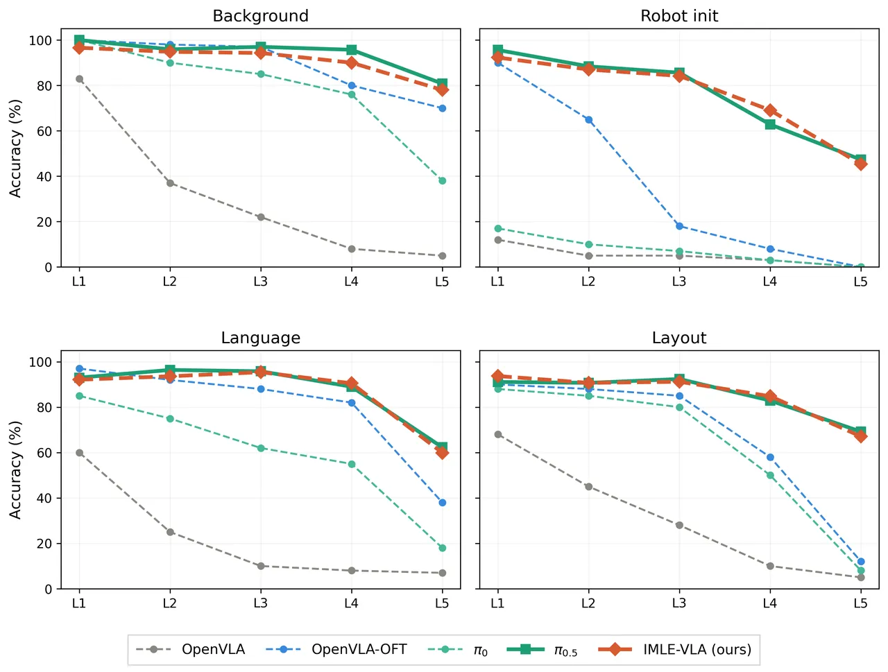
Figure 2 (paper Fig. 2): LIBERO-plus robustness under distribution shift. Success across four perturbation dimensions (background, robot initial state, language, layout), each at five severity levels (L1-L5). Unlike the baselines, which degrade sharply as severity increases, IMLE-VLA matches $\pi_{0.5}$'s robustness throughout; OpenVLA-OFT's drop is consistent with the known limitation of its L1 regression objective.

The sample-factor ablation (paper Fig. 4) reports LIBERO success across all four suites at $H{=}10$ for $m \in \{1, 2, 5\}$. At $m{=}1$ the assignment is trivial, cIMLE reduces to standard L2 regression with no mode-covering guarantee, and a clear performance drop appears. That result empirically confirms the theoretical argument of Eqs. (5) and (6), and matches the limitation OpenVLA-OFT acknowledges for L1 regression. At $m{=}2$ the mode-covering property activates and performance recovers substantially; increasing to $m{=}5$ yields nearly identical results, indicating diminishing returns. The paper therefore uses $m{=}2$ throughout, achieving strong performance while minimizing the per-step cost of generating additional candidates.

The LIBERO-plus robustness results are, in my assessment, the most consequential in the paper. LIBERO-plus applies systematic test-time perturbations to LIBERO tasks across four axes (background, robot initial state, language, layout) at five severity levels (L1-L5). Across all axes and severities, IMLE-VLA retains $\pi_{0.5}$'s robustness, while all other baselines exhibit larger drops as severity increases, with OpenVLA-OFT degrading most sharply. The authors attribute this to the objective: cIMLE enforces mode coverage by construction and therefore avoids the collapse-to-median failure mode. Put differently, what breaks first under distribution shift is not the model with the smaller backbone but the model whose objective collapses modes. A 3B backbone holds up under perturbation here while a 7B one does not.

5. Real robot: Franka Panda with an A6000, four tasks, four wins

Real-world evaluation compares against the $\pi_{0.5}$ baseline (canonical JAX implementation) on a Franka Emika Panda with an NVIDIA A6000 GPU and two camera views (wrist and scene). Both policies are trained on DROID and deployed zero-shot on four tabletop manipulation tasks, with success reported over 20 episodes per task. $\pi_{0.5}$ runs at a 15 Hz control frequency while IMLE-VLA operates at 55 Hz. The authors are explicit about the horizon choice: unlike LIBERO's deterministic contact dynamics, real-world manipulation introduces physical uncertainty such as grasp slippage and surface friction variation, requiring more frequent replanning. They therefore adopt the $\pi_{0.5}$ default horizon ($H{=}8$) and extend IMLE-VLA to $H{=}12$, since the faster inference compensates for the longer horizon while still yielding a shorter wall-clock replan interval than $\pi_{0.5}$.

Task	Ours (of 20)	$\pi_{0.5}$ (of 20)	VLA-WC ours (s)	VLA-WC $\pi_{0.5}$ (s)	Jerk ratio ↓
Pineapple in bowl (single-step)	19	15	18.56	123	$2.7\times$
Swap pineapple and cube (multi-step)	18	15	31.1	178.3	$2.2\times$
Pineapple in cabinet (multi-step, door closing)	15	12	99.4	389.4	$3.0\times$
Pineapple on moving plate (reactive)	16	12	16.7	89.5	$2.7\times$

Table 4 (paper Table V): real-world results on a Franka Emika Panda with an NVIDIA A6000, 20 episodes per task. VLA-WC is wall-clock on VLA forward passes per successful episode, averaged over successful episodes per task; the jerk ratio is $\pi_{0.5}$'s mean proprioceptive jerk divided by ours, so higher means smoother motion relative to the baseline. Across the four tasks VLA-WC drops $3.9\times$-$6.6\times$.

The four tasks span three capability classes: single-step manipulation (grasp a squishy pineapple toy from the table and place it in a bowl), multi-stage sequential reasoning (remove the pineapple from a bowl, then place a red cube inside; or place the pineapple in an open cabinet and close the door), and reactivity to a dynamic environment (a remote-controlled car drives an attached plate across the table, and the robot must place the pineapple on the moving plate, requiring continuous target adjustment). IMLE-VLA outperforms $\pi_{0.5}$ on every task, reduces VLA-only wall-clock by $3.9\times$-$6.6\times$, and completes episodes approximately $2\times$ faster end-to-end (supplementary videos).

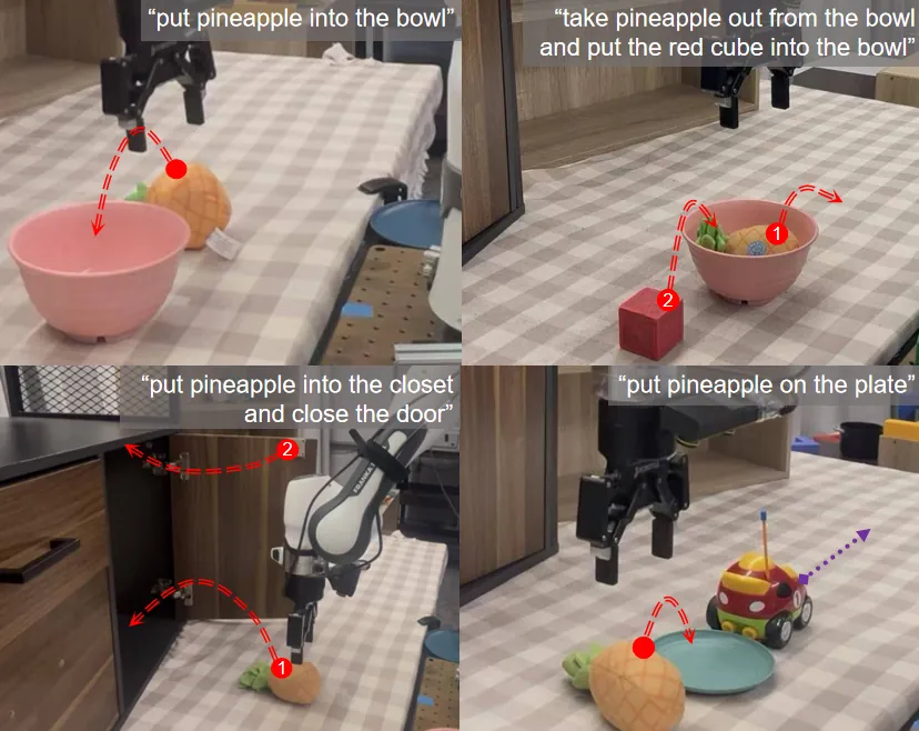
Figure 3 (paper Fig. 5): real-world experiments across three categories, single-step manipulation, multi-step sequential reasoning and dynamic reactivity. IMLE-VLA generates faster, smoother and more successful actions in all three.

Motion quality is quantified as proprioceptive jerk: the third backward finite difference of the measured joint positions (7 arm joints, gripper excluded), normalized by $dt^3$ and averaged over joints and steps. IMLE-VLA reduces mean jerk by $2.2\times$-$3.0\times$ across all four tasks. The physical explanation combines two mechanisms: faster inference minimizes the time the robot idles while the model computes, and a longer execution horizon means fewer replans; together they eliminate the visible stop-wait-execute pauses and abrupt directional corrections that $\pi_{0.5}$ exhibits at each replan. The authors give two concrete observations. On swap pineapple and cube, $\pi_{0.5}$ changes direction repeatedly before each placement while IMLE-VLA follows a direct trajectory and finishes faster. On pineapple in cabinet, when the pineapple slips from the gripper during insertion, IMLE-VLA detects the failure and re-grasps quickly because its replan interval is short.

The reactive task shows the largest gap and makes the latency-to-failure chain explicit. Although IMLE-VLA executes a longer action horizon, its faster inference produces a much shorter wall-clock replanning cycle, so the policy closes the perception-action loop more frequently in real time and can continuously track and adapt to the plate's motion. $\pi_{0.5}$ replans more slowly and therefore acts on increasingly stale observations: by the time a new action sequence is generated, the plate has already moved, so the robot repeatedly reaches toward outdated target locations and ultimately fails. The causal story is clean. This is not a case of a less capable policy but of a policy whose observations have expired before they are used.

Limitations

Stated by the authors: a longer execution horizon trades reactivity for throughput. In the horizon ablation the paper says plainly that extending $H$ still trades reactivity for throughput, because the robot executes more actions before conditioning on a new observation. The $11.0\times$ throughput figure comes from $H{=}30$, the same configuration where success falls from 98.0% to 97.1%. More importantly, that cost is amplified in fast-changing environments, and the paper's own moving-plate task demonstrates that the closing frequency of the perception-action loop determines success or failure, while $H{=}30$ means 30 open-loop actions between observations. No mechanism is offered for adapting $H$ to scene dynamics; in practice $H$ is a hand-set constant (10 or 30 in simulation, 12 on the robot).

Stated by the authors: at $m=1$ the objective degenerates into mean regression. Eqs. (5) and (6) together with the Fig. 4 ablation show that the mode-covering capability of cIMLE depends entirely on $m > 1$. At $m{=}1$ the assignment is trivial, the objective collapses to standard L2 regression, and its minimizer ignores the noise and outputs the conditional mean, with a measurable performance drop. This is a precondition of the method rather than a tunable knob.

Additional observations from a reader's perspective. First, $m{=}2$ means the generator is explicitly trained to cover at most two modes. The near-identical results at $m{=}5$ are used to argue diminishing returns, but they are measured on LIBERO, where genuinely ambiguous decision points (go left or go right around an object) are relatively few. Whether two-mode coverage suffices in settings with heavier ambiguity, such as long-horizon assembly, tool selection among several options, or multiple valid avoidance paths around a human, is not evidenced in the paper.

Second, the drop-in replacement claim is validated only on $\pi_{0.5}$. The conclusion states that because the approach modifies only the action head it can replace the iterative heads of existing VLAs, yet every experiment (Tables I-V) is built on the $\pi_{0.5}$ 3B backbone and its CFM head. Whether models with different capacities and different action-expert structures, such as $\pi_0$, RDT-1B or CogACT, benefit equally is untested, as is the implicit dependency introduced by initializing $G_\theta$ from a checkpoint: a pretrained iterative head must already exist to seed the single-step generator.

Third, the evaluation surface is narrow. Simulation results concentrate on a single benchmark, LIBERO, with 40 tabletop tasks, a single-arm Franka and deterministic contact dynamics, and the robustness evidence comes from LIBERO-plus, a perturbed version of the same tasks. The real-robot suite is also single-arm tabletop work: four tasks at 20 episodes each. Differences such as 19/20 versus 15/20 carry wide confidence intervals at that sample size, and the paper reports no significance testing, cross-seed variance, or failure-mode distribution. Bimanual manipulation, mobile manipulation, loco-manipulation and long-horizon multi-object scenes are all outside coverage.

Fourth, training cost is not reported. The paper argues that training reduces to the action head alone with minimal cost and that cIMLE adds negligible training overhead, but no GPU-hours, step counts, dataset sizes, or head-to-head comparison against CFM training are given. A reader cannot judge how cheap "cheap" is, nor what the candidate generation at $m{=}2$ actually costs at dataset scale.

Fifth, code is not yet available. The abstract states that videos and code are available at the project page, but as of writing that page hosts demo videos only, with no runnable training or inference code, and the metadata record carries no repository URL. The 55 Hz, 98.0% and $11.0\times$ figures cannot currently be reproduced independently, and part of the cross-baseline comparison in Table II is taken from another paper measured on different hardware (H100), adding one layer of indirection to comparability.

Conclusion and Outlook

The contribution decomposes into four layers: problem, objective, instantiation, evidence. At the problem layer, VLA latency is dominated by iterative action generation (10 Euler steps in $\pi_{0.5}$), and system-level optimization cannot lift this algorithmic ceiling, as the flat 15 to 20 to 25 Hz curve shows. At the objective layer, a single-step regression head collapses modes because of its loss, a claim made rigorous by Eqs. (5) and (6) and verified by the $m{=}1$ ablation, so what is needed is an objective that enforces mode coverage by construction; the nearest-neighbour assignment of cIMLE does exactly that by penalizing only the winner and leaving the remaining candidates free to cover other modes. At the instantiation layer, freezing the VLM backbone, training only a head initialized from the $\pi_{0.5}$ checkpoint, using $m{=}2$, computing the VLM embedding once per batch, performing assignment without gradients and backpropagating only through the winner together keep the training overhead negligible. At the evidence layer: 55 Hz ($3.67\times$), 1,650 Hz throughput at $H{=}30$ ($11.0\times$) and a $10.5\times$ VLA-WC reduction; 98.0% on LIBERO, the best average while also leading frequency; retained $\pi_{0.5}$ robustness on LIBERO-plus where other baselines degrade sharply; and four wins out of four on the real robot with $2.2\times$-$3.0\times$ lower jerk and $3.9\times$-$6.6\times$ lower VLA-WC.

Methodologically, the most transferable insight is the decoupling of the speed problem from the distribution-modelling problem. Prior acceleration routes either shrink constants (kernels, quantization, compilation), shrink capacity (distilling into a shallower student), or change the objective while accepting the mode collapse that objective brings (an L1 regression head). IMLE-VLA shows that collapse is not a necessary property of single-step generation but a property of doing single-step generation with a regression loss. Swap the loss for a winner-takes-all assignment and single-step generation and multimodal coverage hold at the same time. That is also why the method stays robust on LIBERO-plus where the 7B-backbone OpenVLA-OFT does not: under distribution shift, the objective that collapses modes fails first, not the smaller backbone.

Looking forward, the authors position IMLE-VLA as a drop-in replacement for the iterative action heads in existing VLAs and as a promising direction toward even faster generalist robot policies. Working backwards from the constraints this paper exposes, the most valuable extensions are: porting the cIMLE head to other VLA families ($\pi_0$, RDT-1B, CogACT) to actually substantiate the drop-in claim; studying the relationship between $m$ and the ambiguity of the task distribution, i.e. an adaptive sample factor rather than a fixed $m{=}2$; turning $H$ from a hand-set constant into a quantity that adapts to environment dynamics, which would directly address the authors' own reactivity caveat; and widening evaluation to bimanual, mobile and long-horizon manipulation while releasing code and training costs so that 55 Hz and 98.0% can be independently reproduced.

Golden Quote

Going from 15 Hz to 55 Hz did not require making those 10 integration steps faster; it required admitting they never had to exist. And the precondition for that admission is understanding why they were there in the first place: generation does not need multiple steps, but single-step generation under a regression loss averages every correct answer into one invalid action. Change the loss and the steps come free.