SkeleWAM: squeezing a manipulation scene into a sparse 3D skeleton

SkeleWAM: Skeleton World-Action Modeling for Efficient Robotic Manipulation
Juyi Sheng, Hua Wang, Mengyuan Liu (Peking University)
arXiv:2610.02120v1 [cs.RO], 1 October 2026 · Project page
Code status: no public code is provided. Neither the arXiv full text nor the project page links a code repository; the project page hosts only the paper PDF, demo videos and images.

One-sentence summary

World action models (WAMs) usually represent future state as video or visual latents, which encode geometry only implicitly and carry appearance information irrelevant to control. SkeleWAM keeps only three kinds of 3D landmarks — robot joints, object centres and interaction points — and uses that sparse skeleton for both action generation and future-skeleton prediction, training with future-geometry prediction as auxiliary supervision and dropping it entirely at inference. On LIBERO-Plus it reaches 85.9% zero-shot success with 57.1M parameters, beating the 2B-parameter Cosmos-Policy by 3.7 points.

1. Background: from VLAs to world action models

Learning-based robotic manipulation has moved quickly from task-specific visuomotor policies to general-purpose robot foundation models. ACT learns action chunks from visual observations, while Diffusion Policy and DP3 model expressive action distributions using 2D and 3D visual representations respectively. As pretraining and robot datasets scale, generalist policies and vision-language-action models — RT-2, Octo, OpenVLA, $\pi_0$, $\pi_{0.5}$ — have demonstrated increasingly broad capabilities across manipulation tasks and environments.

World action models go one step further by jointly modelling robot action generation and future state prediction. The latter supplies extra supervision, teaching the model how a manipulation scene evolves under robot actions. The difficulty lies in how that future state is represented. Many existing WAMs represent future state as generated video or learned visual latents.

The paper presses on that choice with two objections. First, latent prediction is indeed cheaper than explicit video generation, but the information a latent retains is largely shaped by the underlying visual encoder and its pretraining objective rather than by what the task needs. Second, and more fundamentally, compressing visual observations does not by itself isolate the geometric variables that govern interaction: the spatial configuration and relative motion of robot and object remain submerged in appearance.

That leads to a more basic question: can a sparse representation of robot-object structure support effective world action learning while substantially reducing model complexity?

The authors' observation is that whatever matters for control in a manipulation scene can be expressed as a set of sparse 3D landmarks on the robot and the manipulated objects. The robot is represented by the 3D positions of its joints; each object is represented by its centre plus a set of interaction points, where the centre captures overall spatial location and the interaction points identify locations relevant to contact and manipulation.

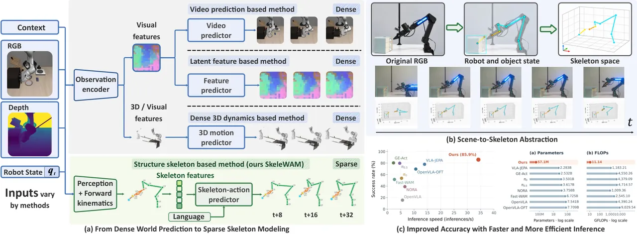
Figure 1: sparse skeleton states enable efficient world action modelling. Existing world action models represent future state as video, visual latents or dense 3D dynamics. SkeleWAM instead converts RGB-D observations and robot state into a sparse 3D skeleton of robot joints, object centres and interaction points, learning action generation and future skeleton prediction jointly.

Each of the three landmark types carries a distinct role: joint positions describe the robot configuration, object centres provide a stable spatial reference, and interaction points mark the contact regions relevant to manipulation. Together they form a complete, appearance-independent skeleton of what can be operated on, which is exactly what the name SkeleWAM — skeleton plus world action model — is meant to signal.

2. Related work, and where SkeleWAM sits

Visuomotor and vision-language-action models. Visuomotor policies learn direct mappings from observations to robot actions. ACT predicts temporally coherent action chunks, while Diffusion Policy and DP3 model multimodal action distributions from image and 3D point-cloud observations respectively. VLA models extend the paradigm by incorporating pretrained vision-language representations for language-conditioned multitask control: RT-2 and OpenVLA adapt vision-language representations to action generation, while $\pi_0$ and $\pi_{0.5}$ improve continuous control and generalisation through flow matching and heterogeneous co-training. More recent work improves policy adaptation, action encoding and model compactness through OpenVLA-OFT, $\pi_0$-FAST and NORA. The shared limitation is that these policies primarily optimise action prediction and do not explicitly model how manipulation scenes evolve under robot actions.

World action models. To capture that evolution, WAMs augment action learning with future state prediction. WorldVLA and UniVLA jointly model action generation and visual world evolution, while DreamZero, GE-Act and Cosmos-Policy leverage pretrained video models for robot control and planning. VLA-JEPA replaces pixel reconstruction with prediction of future latent target representations, and Fast-WAM keeps future video prediction as a co-training objective but removes future generation at inference. As the paper puts it, although latent objectives reduce computational cost and dependence on pixel reconstruction, both videos and visual latents represent interaction geometry only implicitly rather than parameterising it as explicit state variables.

SkeleWAM's positioning follows directly: it defines both current and future states in a sparse 3D skeleton space of robot joints, object centres and interaction points. That lets future geometric prediction supervise representation learning during training without being required for action generation at inference — the same train-time-only co-training idea Fast-WAM used for video, but applied to an explicitly geometric state instead of pixels or latents.

3. Preliminaries: problem formulation

Given a language instruction $\ell$, the current RGB-D observation $o_t$ and the robot proprioceptive state $q_t$, the goal is to generate an action chunk:

$$\mathbf{A}_t = \left[\mathbf{a}_t, \ldots, \mathbf{a}_{t+H_a-1}\right] \in \mathbb{R}^{H_a \times d_a} \tag{1}$$

where $\mathbf{a}_{t+i} \in \mathbb{R}^{d_a}$ is a single robot action, $H_a$ the action horizon and $d_a$ the action dimension. The scene is represented as a sparse 3D skeleton:

$$\mathbf{S}_t = \Phi_{\psi}(o_t, q_t, \ell) \in \mathbb{R}^{N \times 3} \tag{2}$$

with $N$ skeleton nodes and $\Phi_{\psi}$ the skeleton extractor of Section 3.2. Training additionally defines a future skeleton sequence $\mathbf{S}_t^+ = [\mathbf{S}_{t+\delta_1}, \dots]$ used as auxiliary supervision in Section 3.4.

One design choice deserves attention: $\Phi_{\psi}$ has no learnable parameters requiring backpropagation. Robot landmarks come from forward kinematics, and object landmarks are estimated from RGB-D by a pretrained perception network that stays frozen during training. In other words, the skeleton is a state constructed online, not a representation that is learned.

4. Method

4.1 Skeleton world representation

The scene skeleton consists of robot keypoints plus task-relevant object landmarks. For object $m$:

$$\mathbf{P}_{t,m} = \left[\mathbf{c}_{t,m}; \mathbf{u}_{t,m,1}; \ldots; \mathbf{u}_{t,m,L_m}\right] \in \mathbb{R}^{(1+L_m) \times 3} \tag{5}$$

where $\mathbf{c}_{t,m}$ is the object centre and $\mathbf{u}_{t,m,j}$ its $j$-th interaction point. The complete skeleton concatenates these:

$$\mathbf{S}_t = \left[\mathbf{J}_t; \mathbf{P}_{t,1}; \ldots; \mathbf{P}_{t,M}\right], \quad N = N_r + \sum_{m=1}^{M}(1+L_m) \tag{6}$$

with $\mathbf{J}_t \in \mathbb{R}^{N_r \times 3}$ holding robot joint and end-effector positions and $M$ the number of objects; semicolons indicate concatenation along the node dimension. The connections define the skeletal organisation: robot nodes follow kinematic connectivity, and each object centre connects to its own interaction points. Node identities, ordering and connectivity stay consistent over time, and the model predicts node coordinates. All coordinates are expressed in a shared robot-centric frame and normalised with training-set statistics.

The robot-centric frame is worth dwelling on: it means camera viewpoint changes are partially absorbed into the representation. The ablation section later provides direct evidence — 93.4% success under camera perturbation, the best of any method compared.

3.2 Two-expert architecture and the block attention mask

The language instruction is encoded as $\mathbf{C}^\ell = \mathcal{E}_{\mathrm{lang}}(\ell)$. Three separate input adapters map the current skeleton, the noisy action chunk and the noisy future skeleton sequence to tokens:

$$\mathbf{X}_t^c = \phi_c(\mathbf{S}_t), \quad \mathbf{X}^a_{t,\tau_a} = \phi_a(\widetilde{\mathbf{A}}_{t,\tau_a}), \quad \mathbf{X}^s_{t,\tau_s} = \phi_s(\widetilde{\mathbf{S}}^+_{t,\tau_s}) \tag{7}$$

where $\tau_a$ and $\tau_s$ are noise times, distinct from the environment timestep $t$. The current skeleton is never perturbed by generative noise — it always serves as a clean condition.

The architecture follows the two-expert Mixture-of-Transformers design of Fast-WAM: a world expert processes current and future skeleton tokens with shared parameters, while an action expert processes action tokens; both are conditioned on $\mathbf{C}^\ell$. For the three token groups ordered as $(\mathbf{X}_t^c, \mathbf{X}^a_{t,\tau_a}, \mathbf{X}^s_{t,\tau_s})$, the block attention mask is:

$$\mathbf{M} = \begin{bmatrix} 1 & 0 & 0 \\ 1 & 1 & 0 \\ 1 & 0 & 1 \end{bmatrix} \tag{8}$$

Rows index query groups and columns index key and value groups, with 1 meaning allowed and 0 blocked. Current skeleton tokens attend within their own group. Each prediction group attends to the current skeleton and to itself, with no attention between action and future-skeleton tokens. The output heads predict vector fields $\hat{\mathbf{v}}^a_\theta \in \mathbb{R}^{H_a \times d_a}$ and $\hat{\mathbf{v}}^s_\theta \in \mathbb{R}^{H_s \times N \times 3}$ in a single forward pass.

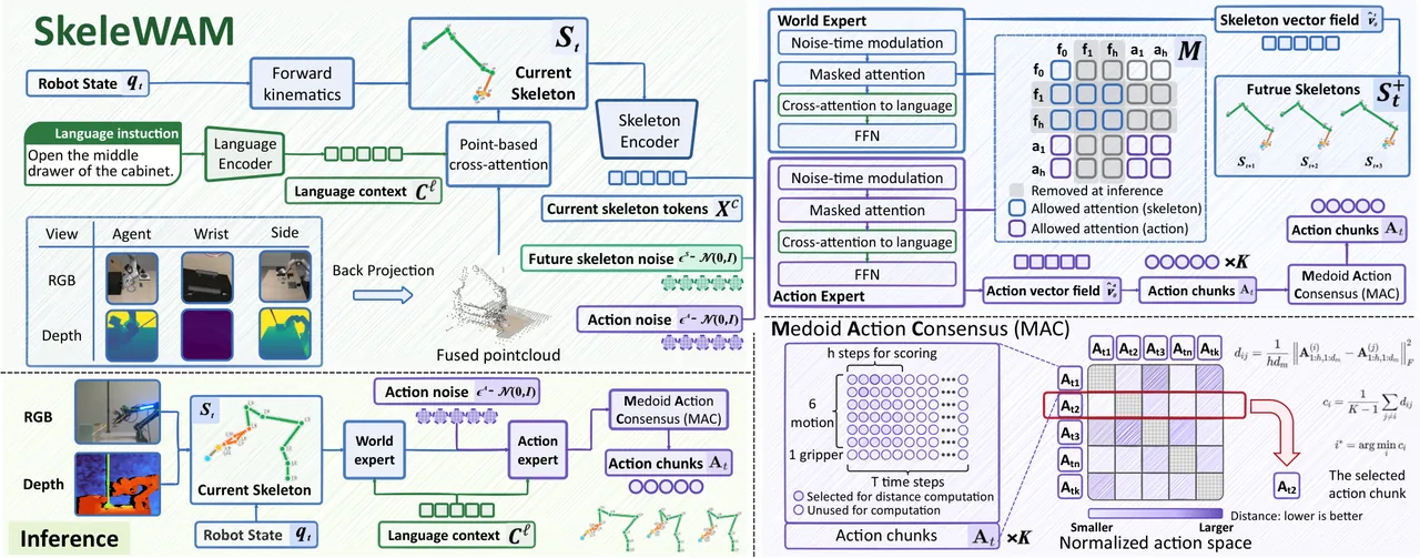
Figure 2: SkeleWAM overview. Frozen visual perception and forward kinematics construct the current skeleton; action generation and future skeleton prediction share the world expert, and only the former is kept at inference.

3.3 Training objective: flow matching with joint supervision

Both prediction tasks are trained with flow matching. Given a demonstration pair $(\mathbf{A}_t, \mathbf{S}_t^+)$, standard Gaussian noise $\boldsymbol{\epsilon}^a$, $\boldsymbol{\epsilon}^s$ of matching shape is sampled together with noise times $(\tau_a, \tau_s) \sim \rho$ on $[0,1]^2$. The interpolation paths are linear:

$$\widetilde{\mathbf{A}}_{t,\tau_a} = (1-\tau_a)\mathbf{A}_t + \tau_a\boldsymbol{\epsilon}^a, \quad \widetilde{\mathbf{S}}^+_{t,\tau_s} = (1-\tau_s)\mathbf{S}^+_t + \tau_s\boldsymbol{\epsilon}^s \tag{9}$$

with noise time 0 corresponding to data and 1 to Gaussian noise. The target vector fields are noise minus data:

$$\mathbf{v}^a = \boldsymbol{\epsilon}^a - \mathbf{A}_t, \qquad \mathbf{v}^s = \boldsymbol{\epsilon}^s - \mathbf{S}^+_t \tag{10}$$

The joint objective has two terms, with the skeleton term weighted by $\lambda_s$:

$$\mathcal{L}_{\mathrm{action}} = \mathbb{E}\left[\operatorname{MSE}\left(\hat{\mathbf{v}}^a_\theta, \mathbf{v}^a\right)\right], \quad \mathcal{L}_{\mathrm{skeleton}} = \mathbb{E}\left[\operatorname{MSE}\left(\hat{\mathbf{v}}^s_\theta, \mathbf{v}^s\right)\right] \tag{11}$$

$$\mathcal{L} = \mathcal{L}_{\mathrm{action}} + \lambda_s \mathcal{L}_{\mathrm{skeleton}}$$

There is a structural point here: both losses update the world expert. The skeleton loss supervises future geometric prediction, while the action loss propagates through the current-skeleton path. Future skeleton prediction is therefore not a parallel auxiliary head; it shapes the shared representation the action expert depends on. That is why ablating it costs 5.8 points, as Section 4.4 shows.

3.4 Inference and Medoid Action Consensus

At inference the current skeleton path and the action expert are kept while future skeleton tokens are omitted. Starting from pure Gaussian noise, the learned action vector field is integrated:

$$\frac{\mathrm{d}\widetilde{\mathbf{A}}_{t,\tau}}{\mathrm{d}\tau} = \hat{\mathbf{v}}^a_\theta\left(\widetilde{\mathbf{A}}_{t,\tau}, \tau; \mathbf{S}_t, \ell\right), \qquad \tau: 1 \rightarrow 0 \tag{12}$$

and the integration result is the sampled action chunk $\mathbf{A}_t = \widetilde{\mathbf{A}}_{t,0}$.

Because sampling is stochastic, the paper proposes Medoid Action Consensus (MAC) as a lightweight way to choose among candidates. Given $K \ge 2$ candidates generated from independent noise initialisations, candidates are compared over their first $h \le H_a$ steps and $d_m$ continuous motion dimensions in normalised action space:

$$d_{ij} = \frac{1}{h d_m} \left\|\left(\mathbf{A}^{(i)}_t\right)_{1:h,1:d_m} - \left(\mathbf{A}^{(j)}_t\right)_{1:h,1:d_m}\right\|_F^2 \tag{13}$$

MAC selects the candidate with the smallest average dissimilarity, i.e. the medoid of the trajectory set:

$$c_i = \frac{1}{K-1}\sum_{j \neq i} d_{ij}, \qquad i_{\mathrm{sel}} = \arg\min_i c_i, \qquad \mathbf{A}^{\mathrm{MAC}}_t = \mathbf{A}^{(i_{\mathrm{sel}})}_t \tag{14}$$

MAC's practical virtues are real: it requires neither a reward model nor a value model, and it avoids averaging potentially incompatible trajectories — which matters for manipulation, where averaging two individually plausible trajectories often yields a third implausible one. Note the complete selected chunk is retained, including dimensions excluded from the distance computation. Execution takes the first $H_e \le H_a$ actions, updates the skeleton from the latest observation, and replans. $H_e$ controls replanning frequency while $h$ is used only for candidate selection.

flowchart TD
    I[RGB-D observation o_t + proprioception q_t] --> P[frozen perception
object centres and interaction points]
    J[forward kinematics
joints and end-effector] --> S[current sparse skeleton S_t]
    P --> S
    L[language instruction] --> E[encoded as C^l]
    S --> M[Mixture-of-Transformers
world expert + action expert]
    E --> M
    N[Gaussian noise] --> M
    M --> A[K action chunk candidates]
    A --> MAC[MAC: pick the medoid
Eq.13-14]
    MAC --> EX[execute first H_e steps]
    EX --> I
    M -.training only.-> FS[future skeleton prediction
auxiliary supervision Eq.11]

5. Experiments

5.1 Setup

Evaluation uses the full LIBERO-Plus benchmark: 10,030 variants across seven perturbation categories, reporting zero-shot task success without fine-tuning on the evaluation variants. Training and evaluation run on a single NVIDIA RTX 4090 for 60K steps at an effective batch size of 48, jointly predicting $H_a = 32$ action steps and eight future skeleton states. Inference uses 10 flow-integration steps, executes $H_e = 16$ actions before replanning, samples $K=3$ MAC candidates with consensus over their first $h=10$ motion steps, and omits future skeleton prediction entirely.

Baselines cover VLA policies (OpenVLA, OpenVLA-OFT, NORA, UniVLA, $\pi_0$, $\pi_0$-Fast, $\pi_{0.5}$) and methods with world modelling or future-state prediction (WorldVLA, Fast-WAM, VLA-JEPA, GE-Act, Cosmos-Policy). A privileged variant, SkeleWAM (sim-state), takes object coordinates directly from simulator state, bypassing visual object localisation.

5.2 Simulation results

Method	Params	Camera	Robot init	Language	Light	Background	Noise	Layout	Overall
OpenVLA	≈7.5B	0.8	3.5	23.0	8.1	34.8	15.2	28.5	15.6
OpenVLA-OFT	≈7.7B	56.4	31.9	79.5	88.7	93.3	75.8	74.2	69.6
NORA	≈3.8B	2.2	37.0	65.1	45.7	58.6	12.8	62.1	39.0
UniVLA	≈7B	1.8	46.2	69.6	69.0	81.0	21.2	31.9	43.9
$\pi_0$	≈3.5B	13.8	6.0	58.8	85.0	81.4	79.0	68.9	53.6
$\pi_0$-Fast	≈3B	65.1	21.6	61.0	73.2	73.2	74.4	68.8	61.6
$\pi_{0.5}$	≈3.6B	70.6	50.5	84.4	95.7	93.4	87.4	84.1	79.7
WorldVLA	≈7B	0.1	27.9	41.6	43.7	17.1	10.9	38.0	25.0
Fast-WAM	≈6.7B	16.4	44.5	68.9	78.2	53.7	37.7	60.7	51.5
VLA-JEPA	≈2.3B	64.2	67.7	88.1	91.8	93.4	65.8	83.9	77.9
GE-Act	≈2.5B	60.7	77.0	77.4	95.8	86.0	90.9	80.2	80.3
Cosmos-Policy	≈2B	75.8	63.3	81.7	96.5	88.9	92.7	82.2	82.2
SkeleWAM (ours)	≈57.1M	93.4	71.9	89.1	96.0	93.9	66.6	85.9
SkeleWAM (sim-state) §	≈51.4M	96.1	75.2	89.0	96.6	96.7	69.0	87.7	87.7

Table 1: zero-shot success rates (%) on LIBERO-Plus, 20 trials per task. § denotes privileged simulator input.

The parameter comparison is the most striking thing in this table. SkeleWAM reaches 85.9% overall with 57.1M parameters, while the strongest observation-based baseline Cosmos-Policy reaches 82.2% with roughly 2B — about 35x fewer parameters and 3.7 points higher success. That directly supports the paper's central claim: representing future state as sparse geometry rather than visual latents can cut model complexity by orders of magnitude.

Column by column, the advantage concentrates on geometry-independent perturbations. Camera robustness is 93.4%, 17.6 points above Cosmos-Policy; language 89.1%, light 96.0% and background 93.9% are all the best observation-based results. The paper's reading is that expressing robot and object state in a shared robot-centric frame effectively removes viewpoint and appearance variation from the state, which is why these perturbations barely dent the policy.

The one weak column is layout, at 66.6%, clearly below $\pi_{0.5}$'s 84.1%. The paper is candid: sparse geometric observations alone do not fully address generalisation to substantially different spatial arrangements. Notably the sim-state variant, which reads coordinates straight from the simulator and bypasses visual localisation, reaches only 69.0% — so the difficulty is not visual localisation but the policy's own generalisation to novel spatial configurations. That moves the problem from perception to generalisation, and it is the single most important self-qualification in the paper.

The overall sim-state gap over RGB-D is just 1.8 points (87.7 against 85.9), with camera and robot-initial-state robustness higher by 2.7 and 3.3 points and language performance on par (89.0 against 89.1). The authors conclude that the frozen perception network already provides effective skeleton estimates, while leaving room for improvement.

5.3 Real-world results

The real platform is an ARX R5 robot with external and wrist-mounted RealSense cameras, working in a tabletop space with a drawer unit, blocks and bowls. Each method is evaluated over five tasks with 20 trials per task.

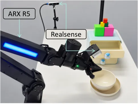
Figure 4: real-world experimental setup. An ARX R5 robot with external and wrist-mounted RealSense cameras operates in a tabletop workspace containing a drawer unit, blocks and bowls.

Method	Open Drawer	Close Drawer	Stack Blocks	Stack Bowls	Put Block in Drawer	Average ↑
Fast-WAM	80	85	80	85	85	83
$\pi_{0.5}$	80	80	70	75	75	76
Cosmos-Policy	85	85	90	90	85	87
SkeleWAM (ours)	80	90	90	95	90	89

Table 2: success rates (%) on five real-world manipulation tasks, 20 trials per task; Average is the unweighted mean across tasks.

SkeleWAM reaches 89% average success, exceeding Cosmos-Policy, Fast-WAM and $\pi_{0.5}$ by 2, 6 and 13 points respectively, and is best or joint-best on four of the five tasks. Notably its 80% on opening the drawer is below every baseline — the one task type where the skeleton representation may be working against it, which the ablations below duly expose.

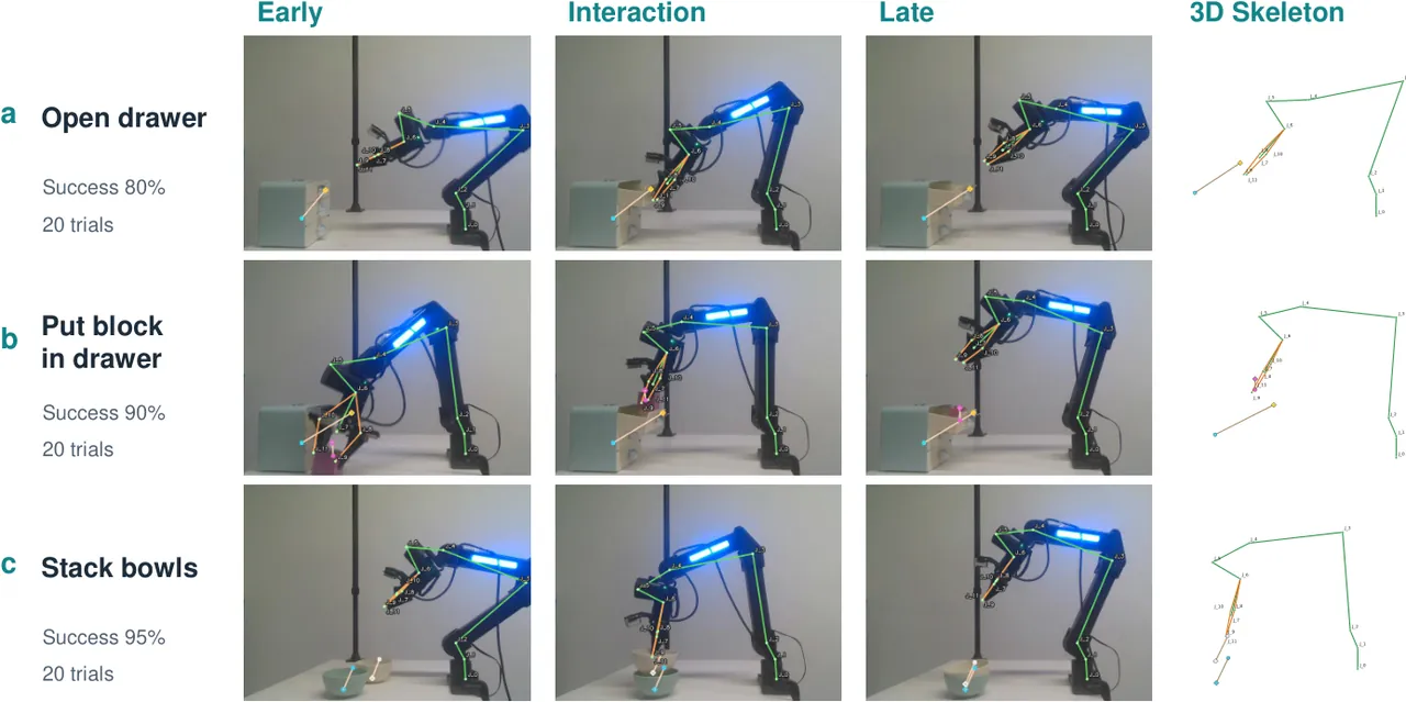
Figure 3: qualitative real-world results. Representative rollouts for opening a drawer, placing a block in a drawer and stacking bowls; each row shows the early, interaction and late stages of a successful rollout together with the corresponding sparse 3D skeleton.

5.4 Ablations

Six design choices are ablated, with training data, optimisation settings and evaluation variants fixed, and defaults $H_a=32$, $H_e=16$, $K=3$, $h=10$.

Configuration	Success (%)
(a) Object skeleton composition
Centres only	82.3
Interaction points only	77.7
Centres + interaction points (default)	85.9
(b) Training objective
Action only	80.1
Action + future skeleton (default)	85.9
(c) Cross-branch attention
No cross-branch attention (default)	85.9
Future skeleton → action	85.6
Action → future skeleton	84.8
(d) Action execution horizon
5 steps	80.7
16 steps (default)	85.9
32 steps	81.8
(e) Number of MAC candidates $K$
1 (no MAC)	84.2
3 (default)	85.9
5	85.2
10	84.1
(f) Consensus window $h$
3	85.3
5	85.4
10 (default)	85.9
16	85.7

Tables 3 and 4: model-side and inference-side ablations, all on the full LIBERO-Plus benchmark in the RGB-D setting.

Three conclusions deserve separate reading.

Object centres and interaction points are individually insufficient. Centres only gives 82.3, interaction points only 77.7, both together 85.9. The two carry complementary information: centres give a stable spatial reference while interaction points describe manipulation-relevant regions. Dropping interaction points costs most (-8.2), which suggests that without a stable spatial reference the interaction points alone cannot even be located.

Future skeleton prediction is worth a real 5.8 points (85.9 against 80.1). Because both variants use the same action-only inference procedure, those 5.8 points come entirely from auxiliary supervision during training; the paper's reading is that predicting future geometric states pushes the shared world expert towards representations that help action generation. Ablation (c) sharpens this: cross-branch attention contributes differences of only about 0.3 points (85.9 / 85.6 / 84.8), far less than removing the auxiliary loss. Together these say the benefit comes from co-training through the shared world expert rather than direct information exchange between the two prediction branches. A useful consequence is that no cross-branch attention is needed, so the future-skeleton branch can be removed entirely at inference.

MAC helps, but not monotonically. $K=1$ (no MAC) gives 84.2 and $K=3$ reaches 85.9, but $K=5$ falls to 85.2 and $K=10$ drops to 84.1 — performance does not increase monotonically with the sampling budget. The consensus window $h$ from 3 to 16 varies by only 0.6 points (85.3 / 85.4 / 85.9 / 85.7), which is robust. The explanation is reasonable: with more candidates the medoid is increasingly likely to land on a middle trajectory that nobody is especially good at.

6. Limitations

The authors' first stated limitation is also the most important sentence in the paper: a performance gap remains under large layout changes, which indicates that sparse geometry alone does not fully capture the variation required for spatial generalisation. Future work is listed as uncertainty-aware perception, adaptive interaction landmarks, and richer relational structure, while preserving the compactness of the skeleton representation.

The authors' second stated limitation is that object landmarks are estimated by a frozen pretrained perception network. The honest number here is that the privileged sim-state variant beats RGB-D by only 1.8 points overall (87.7 against 85.9), so the frozen perception is already good enough — but sim-state is still ahead by 2.7 and 3.3 points on camera and robot-initial-state perturbations, meaning perception error does exist, it simply is not the current bottleneck.

A third observation of my own: the whole pipeline leans hard on the assumption that an object can be described by a fixed set of interaction points. The $L_m$ interaction points are defined offline and the topology — who connects to whom — is fixed. Listing "adaptive interaction landmarks" as future work is precisely an admission that the current version cannot handle contact modes it has never seen, such as grabbing a handle edge that was never annotated, or applying force from a different body part. In addition, the skeleton is constructed from the current observation only and carries no history, so facts like "the drawer has already been opened" must be maintained implicitly through replanning; the paper also does not report error accumulation on long-horizon tasks.

A fourth point about evidence strength: the real-world evaluation has five tasks with 20 trials each, and every number in that table is a multiple of five — which means a single trial is one percentage point. The 89-against-87 gap is two trials. The paper reports this transparently (20 trials per task, unweighted mean), but the real-world 2-point lead should be read as directional evidence rather than a statistically significant result. The simulation side, with 10,030 variants, is considerably more solid.

7. Conclusion and outlook

SkeleWAM's contribution reduces to one sentence: the state space of a world action model need not be video or visual latents — a sparse robot-object 3D skeleton suffices, and it is two orders of magnitude cheaper. Concretely, it replaces dense visual representation with joints, object centres and interaction points, letting a 57.1M-parameter model beat the 2B-parameter Cosmos-Policy on LIBERO-Plus and lead three baselines on real hardware at 89% average success.

A practical implication of the composition ablation deserves mention, because it is a cost the paper does not price. Interaction points are defined offline per object, so someone has to annotate them, and the 8.2-point drop when they are removed says that annotation is not optional bookkeeping. Whether this pays off depends on the setting: for a fixed object repertoire reused across thousands of trials, annotating interaction points once is cheap and buys the largest single ablation gain in the paper. For a deployment with novel objects every session, that upfront cost lands on every new object, and the frozen perception network must supply points it was never trained to predict. This is a plausible second reason why the drawer-opening task, where the grasp target is a handle rather than an object centre, is the one real-world task where the skeleton does not beat every baseline.

Two negative results are more interesting than the headline. First, cross-branch attention barely matters (about 0.3 points), while joint training on the shared world expert matters a great deal (5.8 points) — meaning a simpler architecture, with one branch simply removed at inference, is sufficient. Second, increasing MAC candidates to 10 makes results worse, which is not obvious a priori and says the centre of a set of stochastic trajectories is not necessarily better than a single trajectory.

On parameter efficiency, it is worth being precise about what is actually saved. The 35x gap against Cosmos-Policy is not a smaller backbone in the usual sense. The state itself is what shrank: a sparse skeleton of a few dozen 3D points replaces a dense visual representation, and everything downstream — the input adapters, the shared world expert, the action expert — operates on sequences two to three orders of magnitude shorter than pixels or video latents. Attention cost is quadratic in sequence length, so the saving compounds twice: fewer parameters and cheaper attention. That is also why a single RTX 4090 suffices for training — a structural consequence of the representation rather than a weak result — and why the frozen perception network is tolerable at all: the representation is small enough that perception error does not compound through a deep encoder stack. The design bet is that for manipulation, geometry is a bottleneck for data and compute, not for model capacity — and the layout ablation is exactly where that bet starts to show its limit.

The open question is sharp: layout perturbation at 66.6% is the most glaring number in the paper, and sim-state reaches only 69.0%, so this is not a perception problem but a policy generalisation problem. The skeleton representation solved "what is in the state"; it did not solve "how does the policy plan in an unfamiliar layout". All three of the paper's proposed directions — uncertainty-aware perception, adaptive interaction landmarks, richer relational structure — point at the same requirement: the skeleton has to stop being an artificially fixed topology and become a learnable structure that reflects task demands.

Golden line

A world action model was never missing a state representation. It was missing the step that peels geometry out of appearance.