PAPER DEEP DIVE
T2-z: Test-Time Optimization of Environment Latents for Robotic World Models
Predicting how the world responds to an action requires more than what can be seen: robots must account for environmental factors that are neither directly observable nor explicitly specified, from physical properties such as friction and mass to human-defined environmental rules. We introduce T2-Z for test-time optimization of environment latents, which augments a robotic world model with a learnable environment latent to condition world predictions. This compact latent captures underlying environmental variation without supervision of what environmental factors exist or what values they take. During training, T2-Z alternates between two stages: a world-model optimization stage that fixes the latents and learns general action-conditioned dynamics across environments; and an environment-latent optimization stage that freezes the world model and optimizes the conditioning latents, allowing latent structure to emerge purely through world prediction. At test time, the world model remains frozen and a newly initialized environment latent is optimized from one or more test-time interactions, adapting the model to previously unseen environmental configurations. Across 7 simulated settings and 4 real-world robotic tasks, T2-Z reduces object prediction error metric from 15.20 to 7.00 and raises action success from 33.73% to 72.96%. Its emergent latents capture structured representations of individual and compounded factors across diverse visual scenes. Ablations further show that T2-Z can efficiently infer environment latents from as little as a single test-time interaction trajectory.
One-sentence summary
T2-z separates a robot world model into shared action-conditioned dynamics and a compact environment latent, then freezes the model at test time and optimizes only that latent from a few real interactions.
Research Context and Motivation
An action-conditioned robot world model predicts how a scene will change after a candidate action. If the prediction is reliable, a robot can compare actions internally instead of trying each one physically. The difficulty is that a single observation does not reveal every property needed to predict the consequence of an action. Surface friction, object mass, joint stiffness, soft-body response, and human-defined interaction rules can all change what happens when the same action is applied to the same visible scene.
The paper calls this hidden variation the environment. It is not merely a visual domain shift. Two scenes may look nearly identical while requiring different dynamics. A model trained across many environments without a mechanism for identifying the current one tends to regress toward an average response. Such a predictor may generate a plausible video and still place an object at the wrong location, report the wrong lamp state, or choose an action that fails in the real world.
One possible response is to supply physical parameters as additional inputs. This requires a task designer to define which factors matter and to obtain their values through instrumentation or system identification. The approach works well inside a controlled benchmark, but it limits the model to factors and ranges anticipated by the designers. It also assumes that every relevant environment rule can be expressed as a physical variable before the model sees it.
A second family uses an amortized history encoder. A neural network receives interaction history and produces a context vector for the world model, policy, or simulator. This makes inference fast after training, but it commits to a learned mapping from histories to environments. If the number or type of test-time interactions differs from training, or if several hidden factors combine in a novel way, the encoder may not represent the evidence well.
T2-z takes a more direct route. It maintains an environment latent for each environment, but it does not supervise that latent with friction, mass, or other semantic labels. The only objective is future prediction through flow matching. During training, the model alternates between learning shared dynamics with latents fixed and fitting each latent with the world model frozen. At deployment, a newly initialized latent is optimized on one or more support trajectories while the entire world model remains frozen.
This decomposition has a practical interpretation. The large model learns rules that are useful across environments. The small latent identifies which version of those rules applies here. Test-time computation therefore searches a 32-dimensional state rather than modifying billions of model parameters. The recovered state can then be reused to predict the outcomes of actions that were absent from the support data.
Problem Formulation and Flow Matching
Let an initial observation be x, an action sequence be a, and future visual observations be y. The shared world-model parameters are θ, and the environment latent is ze. T2-z models the conditional predictive distribution
$$p_{\theta}(\mathbf{y}\mid\mathbf{x},\mathbf{a},\mathbf{z}_{e}).$$
No term in this probability model assigns a predefined meaning to a coordinate of ze. The model is not told that one dimension should encode friction or another should encode gravity. The representation is shaped only by which values help predict observed futures.
The base model is trained with a flow-matching objective. Let yt be the noisy or interpolated future observation at flow time t, and let ut be the corresponding target velocity. If the model predicts velocity vθ, the loss is
$$\mathcal{L}_{\mathrm{FM}}(\theta,\mathbf{z}_{e})=\mathbb{E}\left[\left\|\mathbf{v}_{\theta}(\mathbf{y}_{t},t\mid\mathbf{x},\mathbf{a},\mathbf{z}_{e})-\mathbf{u}_{t}\right\|_{2}^{2}\right].$$
Flow matching turns video prediction into a sequence of velocity-estimation problems along a path from noise or a degraded sample to the target observation. T2-z uses the same objective in three roles: training the shared world model, training per-environment latents, and adapting a new latent at test time.
Each training environment starts with an independently initialized latent:
$$\mathbf{z}_{e}^{(0)}\sim\mathcal{U}(0,1).$$
This initialization matters because it avoids giving different environments an ordered, hand-designed code at the start. Structure must emerge from optimization. The released configurations can use alternative initialization values for particular tasks, but the paper's method and algorithm specify uniform initialization as the general training setup.
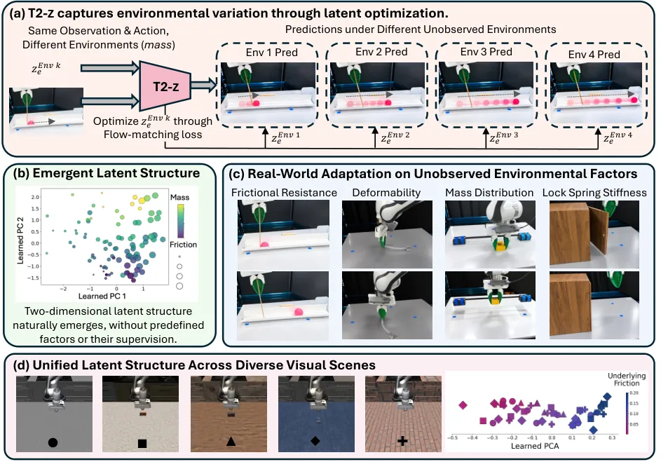
Figure 1 from the paper. The same observation and action can lead to different outcomes under different hidden environments. The principal-component plot shows that learned latents organize according to those differences.
Method
What is shared and what is adapted
The method begins with a model of shared action-conditioned dynamics. Pushing, contact, object persistence, and temporal motion are regularities that can be learned from many environments. T2-z does not assume that these regularities are identical everywhere, but it assumes that most of their structure can be shared while a small latent selects environmental deviations.
The environment latent is deliberately small: one token with 32 dimensions. The world-model backbone is initialized from BWM and uses Wan2.2-TI2V-5B. The diffusion Transformer width is 3072. The contrast between a 32-dimensional environment state and a very large shared backbone is central to the design. It creates an information bottleneck at the point where environment-specific information enters the model.
This bottleneck serves two purposes. It prevents the test-time variable from memorizing a few support videos in a high-dimensional space, and it forces different environments to share the same coordinate system. The ablation that replaces the latent with a directly optimized 3072-dimensional token is therefore not a minor architecture detail; it tests the core hypothesis.
Stage I: learning shared dynamics with latents fixed
In the first training phase, all environment latents are held constant while the world-model parameters are updated. Let De be the trajectory data for environment e. The update in outer cycle k minimizes
$$\theta^{(k+1)}=\arg\min_{\theta}\mathbb{E}_{e,\,(\mathbf{x},\mathbf{a},\mathbf{y})\sim\mathcal{D}_{e}}\left[\mathcal{L}_{\mathrm{FM}}\left(\theta,\mathbf{z}_{e}^{(k)}\right)\right].$$
The model must learn cross-environment dynamics without changing the codes that distinguish environments. It therefore cannot improve simply by moving all latents to a shortcut solution during this phase. The paper begins with 300 world-model updates and uses a learning rate of 10-5, making this the slow branch of adaptation.
Stage II: fitting the environment code with the model frozen
The second phase reverses which variables are allowed to change:
$$\mathbf{z}_{e}^{(k+1)}=\arg\min_{\mathbf{z}_{e}}\mathbb{E}_{(\mathbf{x},\mathbf{a},\mathbf{y})\sim\mathcal{D}_{e}}\left[\mathcal{L}_{\mathrm{FM}}\left(\theta^{(k+1)},\mathbf{z}_{e}\right)\right].$$
With θ fixed, reducing prediction error requires the latent to explain something about the current environment. If the object moves farther because of low friction, the gradient on the latent points toward a code that makes the frozen model generate a longer trajectory. If a hidden rule reverses the meaning of a button action, the latent must move to a region that changes the predicted state transition.
The environment latent uses a learning rate of 0.03. The difference from the world-model learning rate is more than five orders of magnitude. This is the paper's slow-fast decomposition: shared dynamics change gradually, while environment-specific variables move quickly to fit newly observed interactions.
Training alternates the two phases. The paper's default schedule performs 200 latent updates and 200 model updates after the initial model warm-up. A better world model produces cleaner gradients for the latent, and a more informative latent makes the next model update less ambiguous. The goal is not joint minimization in a single step, which the ablation later shows performs worse.
flowchart TD
    A["Training environments"] --> B["Initialize one latent per environment"]
    B --> C["Stage I: freeze z, update world model"]
    C --> D["Stage II: freeze world model, update z"]
    D --> E{"Alternation complete?"}
    E -->|No| C
    E -->|Yes| F["Frozen shared world model"]
    F --> G["New test environment"]
    G --> H["Collect one or two support trajectories"]
    H --> I["Randomly initialize one test latent"]
    I --> J["40 latent-only flow-matching updates"]
    J --> K["Reuse adapted latent for unseen actions"]
Method flow reconstructed from Section 3 and Algorithm 1. Test-time adaptation updates neither a history encoder nor any world-model weights.
Injecting the latent through two conditioning paths
A compact latent is useful only if the backbone can consume it in a way that changes both attention and layer-level modulation. T2-z therefore uses two separate bias-free projectors. Each projection maps the 32-dimensional latent through a 128-dimensional hidden layer to the 3072-dimensional model width, with layer normalization and GELU.
For a path b, the projected value can be written as
$$q_{b}(\mathbf{z}_{e})=W_{b2}\operatorname{GELU}(W_{b1}\operatorname{LN}(\mathbf{z}_{e})),\quad b\in\{\mathrm{token},\mathrm{mod}\}.$$
The token path is concatenated with the action token sequence:
$$C_{e}=[q_{\mathrm{token}}(\mathbf{z}_{e});A_{\mathrm{token}}(\mathbf{a})].$$
The resulting sequence participates in cross-attention. The environment token can thus interact with visual and action information as a distinct conditioning element. The modulation path does something different. It is added to timestep and action modulation:
$$\tilde{\mathbf{b}}_{t}=\mathbf{b}_{\mathrm{time}}+\mathbf{a}_{\mathrm{mod}}+q_{\mathrm{mod}}(\mathbf{z}_{e}),\qquad M=\operatorname{TimeProj}(\tilde{\mathbf{b}}_{t}).$$
The projection produces six adaptive-normalization vectors. In plain terms, the token path changes which condition is visible to attention, while the modulation path changes how strongly different layers respond to that condition. Using separate MLPs prevents the two functions from competing inside a single projection.
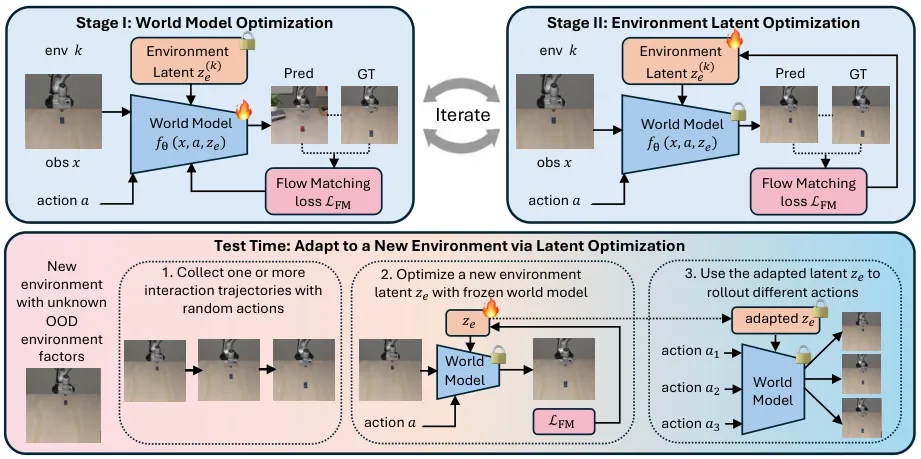
Figure 3 from the paper. Training alternates model and latent optimization. At deployment, only a new latent is optimized and then reused for new actions.
Test-time optimization without a history encoder
At test time, the robot collects support interactions
$$\mathcal{D}_{\mathrm{test}}=\{(\mathbf{x}_{i},\mathbf{a}_{i},\mathbf{y}_{i})\}_{i=1}^{N}.$$
These tuples can come from randomly sampled actions in the new environment. T2-z initializes a test latent and keeps the trained world model fixed. The update is
$$\mathbf{z}_{\mathrm{test}}^{(s+1)}=\mathbf{z}_{\mathrm{test}}^{(s)}-\eta_{z}^{(s)}\nabla_{\mathbf{z}_{\mathrm{test}}^{(s)}}\frac{1}{|\mathcal{D}_{\mathrm{test}}|}\sum_{(\mathbf{x},\mathbf{a},\mathbf{y})\in\mathcal{D}_{\mathrm{test}}}\mathcal{L}_{\mathrm{FM}}\left(\theta^{*},\mathbf{z}_{\mathrm{test}}^{(s)};\mathbf{x},\mathbf{a},\mathbf{y}\right).$$
There is no recurrent encoder that maps a fixed history window to a latent. The optimization objective itself chooses the code that best explains whatever evidence is available. This makes the number of support trajectories a runtime choice rather than an architectural constant. It also allows the latent to seek values outside the range visited during training, although optimization stability still has to be checked.
The paper uses a coarse-to-fine schedule with learning rates 3.0, 1.5, 0.5, and 0.15, each for ten updates, for a total of 40. Large early steps move the latent toward a useful region; smaller late steps refine it. Most simulation tasks use one support trajectory. Light Switch, Mass Balance, Door Close, and Stick Balance use two.
Reusing the latent for unseen actions
The adaptation is useful only if the latent generalizes beyond the support actions. After optimization, a different action a' is predicted as
$$\hat{\mathbf{y}}'\sim p_{\theta^{*}}(\mathbf{y}\mid\mathbf{x},\mathbf{a}',\mathbf{z}_{\mathrm{test}}^{*}).$$
This is the bridge from environment inference to action selection. The robot can use the adapted model to imagine several candidate futures that were never included in the support set. If the latent had merely memorized observed transitions, the action-selection gains would not be expected to persist.
Correspondence with the released code
The file wan_video_action/models/physical_context.py contains the environment-context module. Lines 52 to 75 define context width, token count, the default context, and two independent bias-free projectors. Lines 128 to 144 return separate token and modulation embeddings. This matches the two-path interface described in the paper.
self.token_projector = BiasFreeMLP(
    context_dim, hidden_dim, model_dim,
    input_norm=input_norm
)
self.mod_projector = BiasFreeMLP(
    context_dim, hidden_dim, model_dim,
    input_norm=input_norm
)
token_emb = self.token_projector(context)
mod_emb = self.mod_projector(context)
The file t2z/inference/ours.py implements support-based adaptation. In lines 505 to 594, the inference path freezes the world-model components, clones the initial context, marks it trainable, accumulates or averages support flow-matching losses, and applies the inner-loop update. Lines 585 to 590 show the gradient scaling, step, and optional context clamping.
context = context0.clone()
context = context.requires_grad_(True)
support_loss = getattr(torch.stack(support_losses),
                       support_loss_reduction)()
context = _clamp_context(
    context - float(inner_lr) * context_grad,
    args,
).detach().requires_grad_(True)
The released task configurations expose physical_context_dim: 32, one context token, the dual mode, model learning rate 1e-5, and latent learning rate 0.03. They also vary initialization and support counts by task. The code therefore confirms the central mechanism, but it should not be read as evidence that every paper experiment used one identical YAML file. The paper gives the experimental protocol, while the configs support per-task reproduction.
Why direct optimization can work
The first reason is that prediction error is a broad supervision signal. A physical factor changes future observations regardless of whether it is continuous, discrete, named, or compounded. Flow matching can compare the predicted future against the observed future and route the discrepancy into the small latent. The method therefore avoids building a physical factor list before training.
The second reason is search-space size. Updating the whole backbone at test time changes a huge number of parameters with limited evidence. Updating a LoRA adapter reduces that number, but still searches many dimensions. Optimizing 32 values is a much smaller inference problem, and the ablation shows that abandoning this bottleneck is catastrophic.
The third reason is modular reuse. Once the latent is inferred, it can condition many action predictions without another adaptation step. This differs from methods that adapt a separate module for each query or keep a test-time memory that must be re-read for every action. The compact state makes reuse natural, provided the frozen model's shared dynamics remain valid.
The assumption is also restrictive. If the hidden difference changes the structure of the dynamics rather than selecting a condition within that structure, a low-dimensional latent may not be enough. Severe sensor changes, a different robot body, or an unmodeled contact mechanism could violate the shared-backbone assumption. T2-z addresses environmental variation, not arbitrary transfer between embodiments.
Experimental Design
The simulation suite contains seven settings. Friction changes how far an object travels after a push. Gravity changes the strength of gravity. Mass Collision changes the mass of colliding objects. Light Switch assigns hidden human-defined rules to a button action. Mass Balance varies mass distribution in a dumbbell-like balancing task. Mass times Friction varies two factors simultaneously. Diverse Backgrounds changes friction across 30 visual scene arrangements.
The real-world suite contains Door Close, Ball Friction, Stick Balance, and Soft Pull. Door Close varies the stiffness of a spring lock. Ball Friction requires predicting a pushed ball with unknown mass. Stick Balance attaches different objects to the ends of a stick. Soft Pull varies the deformation caused by rotating a soft object.
The evaluation reports mean physical error, final-frame physical error, LPIPS, PSNR, and action success. Physical error has task-specific units: pixels for several object-motion tasks, lamp-score error for Light Switch, and degrees for Mass Balance. Real-world tasks use tracked-state pixel error. This heterogeneity means the reported averages are useful for aggregate comparison, while individual task numbers should be interpreted against the task definition.
The baselines are carefully matched to the same world-model backbone. The standard model has no environmental conditioning or adaptation. LoRA TTA adapts attention LoRA parameters from test interactions. DINOv2 Context amortizes a 32-dimensional environment context from history. TTT-KQV adapts fast weights inside the world model. All adaptive baselines receive the same support trajectories as T2-z.
Simulation Results
| Method | Mean physical error | Final-frame error | LPIPS | PSNR | Action success |
|---|---|---|---|---|---|
| Standard world model | 12.8575 | 21.9759 | 0.0574 | 31.185 | 37.9% |
| LoRA TTA | 9.3496 | 17.5336 | 0.0584 | 30.182 | 44.8% |
| DINOv2 context | 8.1546 | 14.8014 | 0.0492 | 31.648 | 51.8% |
| TTT-KQV | 12.9233 | 22.5528 | 0.0585 | 30.815 | 42.1% |
| T2-z | 4.7971 | 7.6682 | 0.0430 | 31.760 | 74.2% |
Table 1, based on the paper's seven-task simulation average. T2-z reduces mean physical error by about 62.7 percent relative to the standard model and raises action success by 36.3 percentage points.
The aggregate result is not explained by image quality alone. T2-z has the best LPIPS, but its PSNR exceeds the standard model by only 0.575 decibels. The larger changes appear in task-relevant object state and final configuration. That pattern is consistent with the intended use of a world model: a visually acceptable video is not enough if it selects the wrong physical outcome.
Individual tasks show the effect of hidden variation. On Friction, mean error falls from 11.0626 to 3.8540 and action success rises from 32.0 to 72.0 percent. On Mass Collision, mean error falls from 21.9329 to 6.4522. On Mass Balance, angular error falls from 1.1844 to 0.6403 degrees and success rises from 40.0 to 80.0 percent. These are settings in which the current environment must be inferred from the consequence of an action.
The DINOv2 context baseline is strong. Its simulation average beats LoRA TTA and TTT-KQV, showing that amortizing a compact context can be competitive. In Gravity, DINOv2 reaches 76.5 percent success and 5.9300 mean error, while T2-z reaches 82.4 percent but 7.3408 mean error. T2-z therefore does not dominate every row. Its advantage is the cross-task average and the behavior on several compounded or rule-dependent settings.
The simulation average also hides substantial task difficulty. Light Switch requires a discrete rule rather than a smooth physical parameter. Diverse Backgrounds tests whether the environment code tracks dynamics instead of appearance. Mass times Friction tests whether one code can represent two changes at once. These cases matter because they probe different explanations for why a compact latent might work.
Real-World Results
| Method | Mean tracked error | Final-frame error | LPIPS | PSNR | Action success |
|---|---|---|---|---|---|
| Standard world model | 19.30 | 38.24 | 0.05194 | 32.80 | 26.47% |
| LoRA TTA | 19.27 | 34.42 | 0.04931 | 32.93 | 43.97% |
| DINOv2 context | 17.50 | 32.04 | 0.04788 | 33.41 | 31.86% |
| TTT-KQV | 18.10 | 35.85 | 0.04694 | 33.66 | 36.24% |
| T2-z | 10.85 | 16.66 | 0.04341 | 33.24 | 70.80% |
Table 2, based on the paper's four-task physical-robot average. T2-z lowers mean tracked error by 43.8 percent, lowers final-frame error by 56.4 percent, and raises success by 44.33 percentage points.
The physical experiments provide the stronger motivation for the method. The standard model succeeds on 26.47 percent of trials on average, while T2-z succeeds on 70.80 percent. Stick Balance jumps from 20.00 to 83.33 percent. Door Close rises from 22.22 to 55.56 percent, and final-frame error drops from 41.22 to 13.47. The latter result shows that the latent can respond to mechanical resistance such as spring-lock stiffness, not only to a smoothly varying surface property.
Soft Pull is an important counterexample. T2-z has mean error 18.71, slightly worse than TTT-KQV at 18.23, and its LPIPS is 0.07580, worse than the other methods. It nevertheless has final-frame error 23.59 versus 29.69 for TTT-KQV and action success 81.82 versus 72.73 percent. The discrepancy shows that frame-averaged perceptual measurements do not fully describe whether an action reaches the goal. It also prevents a claim of universal superiority: soft-body deformation remains a difficult case where competing methods can win on some metrics.
The real-world aggregate improvement is larger than in simulation. The paper interprets this as a sign that uncontrolled physical environments contain more hidden variation than controlled simulators. That interpretation is plausible, but the real-world set has only four tasks and one fixed camera setup, so the result is evidence for this benchmark rather than proof that the benefit grows monotonically with real-world complexity.
Latent Structure and Qualitative Behavior
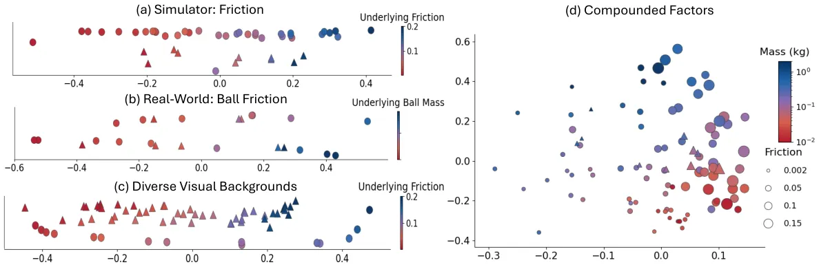
Figure 4 from the paper. Learned environment latents are projected to two principal components. Color and shape are annotations for visualization and were not supplied as supervision.
Figure 4 provides the clearest process evidence in the paper. In simulated friction, latent points form an ordered one-dimensional structure in which color-coded friction values change along the principal direction. The real-world friction task shows a similar organization. Across 30 backgrounds, latents do not simply cluster by visual appearance; scenes with common dynamics share a latent structure. When mass and friction vary together, the projection resembles two axes even though the model was never told that two factors existed.
These plots do not prove that a coordinate has a unique physical meaning. A nonlinear world model can represent several factors in entangled directions, and PCA is only a two-dimensional visualization. The defensible conclusion is narrower: prediction-only optimization produces a representation that is structured with respect to task-relevant hidden variation and is not dominated by background appearance.
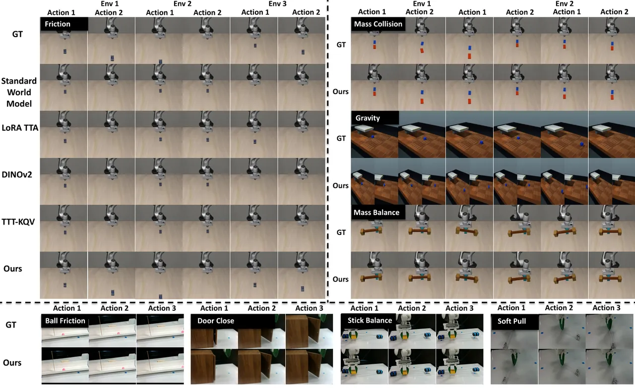
Figure 6 from the paper. The same action applied across environments produces different true outcomes. T2-z more closely follows the environment-dependent motion, while baselines often produce wrong final configurations.
Ablation Studies
| Variant | Mean error | Final error | LPIPS | PSNR | Success |
|---|---|---|---|---|---|
| T2-z | 3.85 | 7.59 | 0.0495 | 31.976 | 72% |
| Joint model-latent training | 7.03 | 15.66 | 0.0657 | 31.203 | 68% |
| Direct 3072-D token optimization | 94.50 | 80.49 | 0.7626 | 15.218 | 24% |
| 32-D random initialization [-0.05, 0.05] | 4.81 | 9.73 | 0.0495 | 32.172 | 60% |
| Alternating budget 100/100 | 5.41 | 11.50 | 0.0484 | 32.208 | 56% |
| Alternating budget 400/400 | 4.31 | 8.80 | 0.0507 | 32.430 | 68% |
Table 3, based on the paper's additional ablation. Directly optimizing a full 3072-dimensional token collapses performance, supporting the low-dimensional bottleneck.
The most informative ablation is the 3072-dimensional direct token. Mean physical error rises to 94.50, LPIPS to 0.7626, and action success falls to 24 percent. A high-capacity latent can fit a small support set while moving the frozen model into a poor region that does not transfer to new actions. The 32-dimensional bottleneck restricts the search toward a reusable environment state.
Joint model-latent training also performs worse, with mean error 7.03 and success 68 percent. When both components move at the same time, the model can reduce loss by changing shared weights instead of isolating environment-specific information. The alternating updates impose a clearer division of labor. The 100/100 schedule is worse than 200/200, while 400/400 is also worse, indicating that balance matters more than simply increasing either phase.
The initialization ablation changes the uniform [0,1] range to a narrow interval around zero. Mean error becomes 4.81 and success falls to 60 percent, below the full model's 3.85 and 72 percent. The optimization can still work, but the starting distribution affects which region is reached within a fixed 40-step budget. This is an optimization detail of practical importance, even though it does not change the central architecture.
Figure 5 further tests the test-time budget and trajectory count. Performance improves up to 40 optimization steps and then largely saturates. Adding support trajectories gives diminishing returns after the task-specific selected count. The result supports the claim that T2-z can infer useful environmental information from very little interaction, but the phrase “very little” remains task-dependent: four harder tasks need two trajectories.
Computational Cost
The appendix reports a compute-only profile on one H200 GPU at a support count of one. T2-z takes 18.09 seconds including latent adaptation and five query generations. LoRA TTA takes 32.73 seconds, and cached TTT-KQV takes 37.57 seconds. The measurement excludes model and sample loading, dataset reads, and MP4 writing.
The comparison is therefore not an end-to-end robot latency claim. It isolates the cost of the adaptation and generation path after inputs are available. Even with that scope, the numbers are useful because they show that optimizing a 32-dimensional state can be cheaper than adapting LoRA weights or fast-weight structures in this implementation.
T2-z still adds an iterative phase that a feed-forward standard model does not have. For a low-latency controller, 40 inner updates may be acceptable if they happen once per environment and their resulting latent is reused, but not necessarily if the environment changes during every control cycle. The right deployment pattern is likely episodic adaptation followed by fast conditioned prediction, with a trigger for re-adaptation when prediction error rises.
Discussion
The conceptual shift in T2-z is from amortization to inference-time solving. A history encoder compresses evidence into a latent with a fixed learned function. T2-z asks which latent best explains the evidence under the current frozen predictor. The latter is less convenient when a low-latency forward pass is required, but it is more flexible when support length or hidden-factor composition differs from training.
The slow-fast separation is also a statement about model maintenance. Shared dynamics should remain stable across environments, while environment identity should be quick to change. This resembles system identification, except the inferred state is not a hand-designed physical parameter. It is an internal code shaped by predictive usefulness. The PCA results suggest that predictive usefulness can create ordered structure, but they do not turn the code into a calibrated physics vector.
The method's scope is therefore specific: a fixed robot and sensing setup, a shared class of dynamics, and hidden environmental conditions that can be observed through action outcomes. Within that scope, the compact latent is a useful interface. Outside it, a latent cannot compensate for missing visual information, a different embodiment, or a contact model that the shared backbone never learned.
The results also raise open questions. How should a robot decide that its current latent is stale? Can uncertainty be represented without abandoning the compact bottleneck? How should support actions be selected to maximize information rather than sampled uniformly? Can multiple latent hypotheses be maintained when observations are ambiguous? The paper demonstrates adaptation quality, but an operational system still needs a policy for collecting evidence and monitoring drift.
Limitations and Boundary Conditions
The paper does not contain a standalone author-written limitations section. The following boundaries are grounded in its experimental setup and released implementation rather than attributed to an explicit self-critique. First, real-world evaluation uses one fixed Intel RealSense D435i main RGB view at 640 by 480 resolution and 20 frames per second. Multi-view perception, camera motion, depth changes, and sensor replacement are not systematically tested.
Second, the evaluation covers seven simulated settings and four physical tasks. It spans friction, gravity, mass, hidden lamp rules, balancing, door stiffness, and soft deformation, but it is not a broad census of open-world robotics. Multi-factor variation is analyzed mainly in simulation. The real-world tasks are designed so that an environment difference has a measurable effect on the action outcome, which may be easier than unconstrained deployment.
Third, test-time adaptation requires observed outcomes. The optimization compares predicted and true futures through flow matching, so the robot needs support trajectories with usable visual results. Self-collected video can provide this evidence, but selecting frames, handling occlusion, and deciding when an interaction is informative remain system-level problems. A test environment that cannot be safely explored may not provide enough support data.
Fourth, the efficiency result is a single-GPU compute profile that excludes loading, data access, and video output. It does not establish real-time performance on a robot's onboard computer. The iterative test-time phase also introduces a different latency profile from a feed-forward encoder. Any deployment claim should be based on end-to-end measurements, including perception, communication, and action execution.
Fifth, the alternating schedule and test-time learning rates are tuned components. The paper studies the number of alternation steps, learning-rate scale, initialization, and optimization budget, and each changes performance. Adapting the method to a new backbone, frame rate, action space, or support length may require another tuning cycle. The compact latent reduces the search dimension but does not remove the need for stable optimization.
Conclusion
T2-z adds a small environment state to a large action-conditioned world model and makes that state the sole target of test-time adaptation. Shared dynamics are learned across environments; the latent explains the current environment without semantic supervision. Alternating training gives the two components distinct roles, while freezing the world model at deployment prevents a few support trajectories from rewriting the whole predictor.
The empirical case is substantial but not universal. Across seven simulation settings, mean physical error falls from 12.8575 to 4.7971 and action success rises from 37.9 to 74.2 percent. Across four real tasks, mean tracked error falls from 19.30 to 10.85 and success rises from 26.47 to 70.80 percent. At the same time, Soft Pull shows that T2-z can lose on mean error and LPIPS, and the evaluation remains narrow relative to open-world deployment.
The most promising implication is architectural rather than purely numerical. A robot world model can expose a dedicated adaptation layer that is small, reusable, and optimized only when the environment changes. The next step is to test whether that layer remains identifiable across cameras and embodiments, whether uncertainty can be attached to it, and whether support actions can be chosen actively instead of sampled. Such work would turn a compelling benchmark result into a dependable deployment mechanism.
SOURCE LINKS