How to Build a Humanoid Robot at Home: The Asimov 1 Build Guide

Tinkerers who want to build a humanoid robot rarely know where to start. They watch Unitree or Figure AI videos, read a few papers, maybe buy a small hobby kit, and then discover an enormous gap between "a robot that does a backflip in a controlled lab" and "a robot I can actually build, modify, and understand." That gap exists because most humanoid robots are closed systems: you cannot see inside them, you cannot source a replacement part in two days, and when you want to change a joint design, you simply cannot.

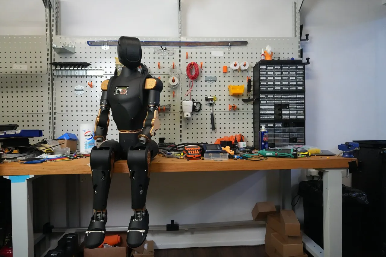
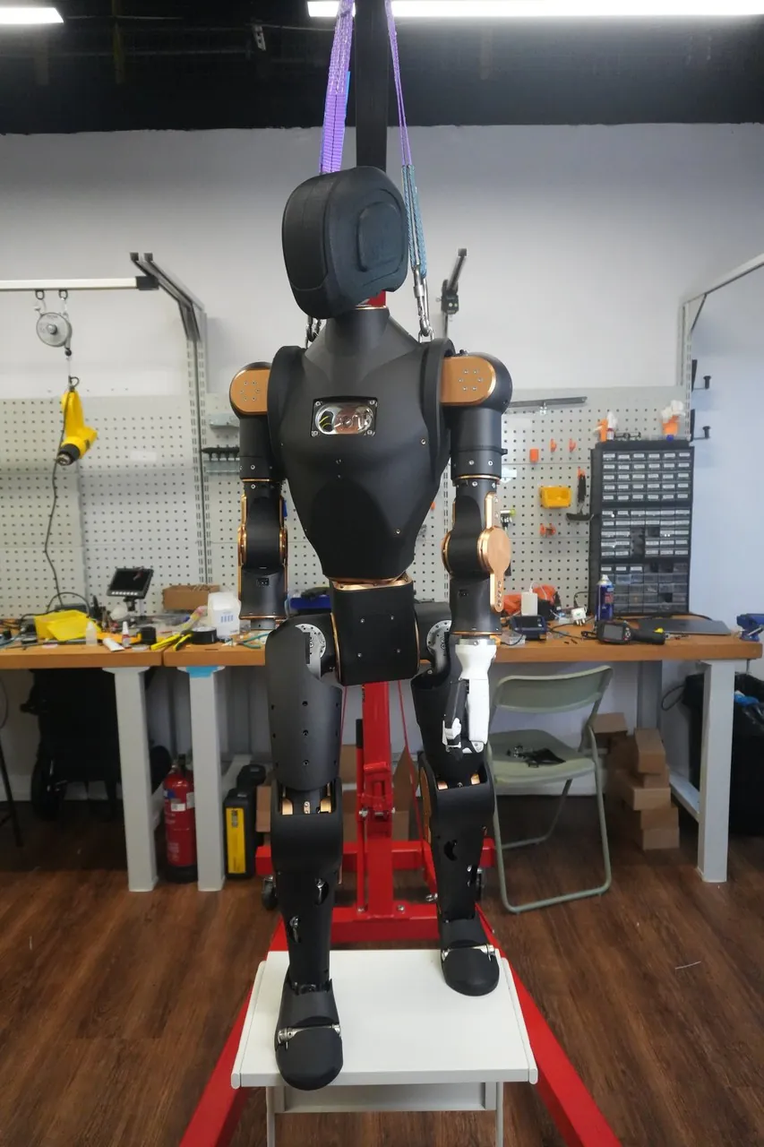
Asimov 1 is a DIY kit that includes everything you need to build a humanoid at home.

This guide, adapted from the build guide published by the Asimov team at Menlo Research, walks through exactly that: the hardware, the fabrication, the electronics, the control stack, and the sim-to-real transfer work that most guides skip. Asimov 1 is a $20,000 kit delivered to your door, shipping since the end of August to customers in more than 20 countries, with the BOM, CAD files, simulation environment, and baseline walking policy all open. It is positioned as the fastest way into humanoid robotics for people who want to be in the room when this technology matures.

What you're building

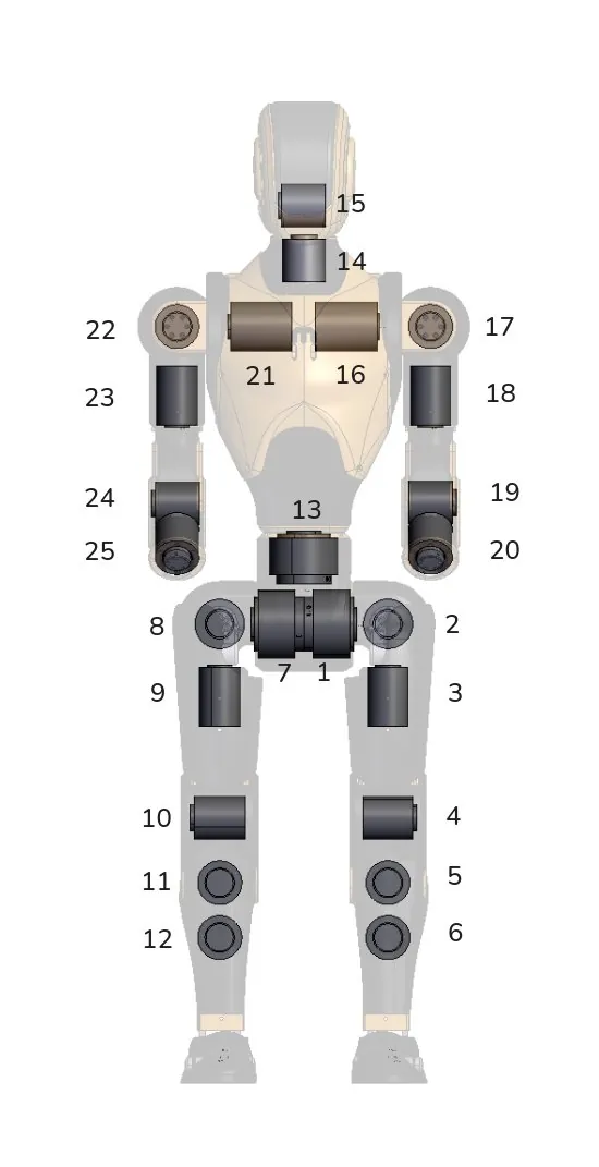
Asimov 1 is 1.2 meters tall, weighs 35 kilograms, and has 25 actuated degrees of freedom: six per leg, five per arm, one at the waist, and two in the neck. It carries an integrated sensor suite, onboard compute, and a baseline locomotion policy that runs on the robot itself.

Property	Specification
Height	1.2 m (head 0.17 m, torso 0.36 m, legs 0.7 m)
Mass	35 kg
Actuated DoF	25 total: 6 per leg, 5 per arm, 1 waist, 2 neck
Actuators	36 Nm units at ankle and neck; 120 Nm units at hip pitch and waist yaw
Ankle mechanism	Parallel RSU linkage (two motors drive pitch and roll through a shared linkage)
Sensors	Monocular camera, IMUs, microphone, speaker, motor joint-state feedback
Compute	Edge board (high-level control), motion control board (internal bus), network board, power distribution board
Build time	~20 hours (down from the 100 hours quoted at launch)
Kit price	$20,000, delivered

What's in the kit

Category	Contents
Hardware	All BOM components unassembled, power supply and cabling, spare parts
Compute	Edge board for high-level control, motion control board for the internal bus, network board, power distribution board
Sensors	Monocular camera, IMUs, microphone, speaker, motor joint-state feedback
Safety	Physical and wireless e-stop, safety guidelines, labels, operating guidelines
Software	Pre-trained walking policy, robot cloud API and CLI, edge API for low-level control, teleoperation app, virtual Asimov digital twin
Docs	Quickstart guide, full assembly manual, DIY video tutorials

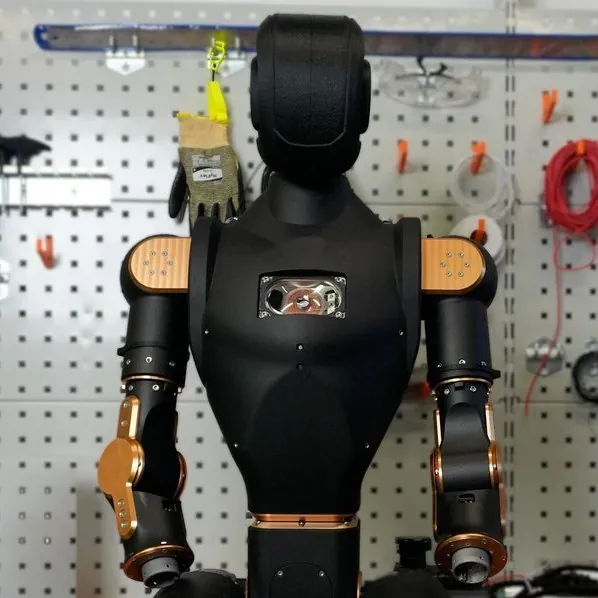
Not included: tools, battery, 4G/5G modules, and premium sensors such as LiDAR or a 360-degree camera. And a fair warning from the team: this is not a toy. In complexity it is closer to a car than to a weekend project.

The build: twenty hours, five systems, one clean power-on

Expect around 20 hours of work. Design updates brought that down from the 100 hours quoted at launch; the work did not get simpler, there is just less of it. A humanoid robot is not a single system but five or six systems that must work together before any of them is useful. The mechanical structure has to be correct before you wire it. The wiring has to be correct before you power it. The power-on has to be clean before you calibrate. The calibration has to be right before simulation means anything.

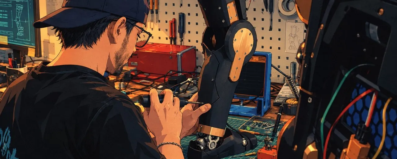
Most people underestimate wiring and bring-up. They expect the hard part to be mechanical assembly, because that is what they can see. In practice the hard part is usually the first power-on: motors that respond in the wrong direction, joints that home incorrectly, CAN IDs that were never set before assembly. These are fixable problems, but they take time, and they require the robot to be in a controlled, safe setup before you find them. Each phase has its own failure modes and you cannot skip ahead. The 20 hours is not assembly time; it is the minimum time required to understand what you built.

The right first milestone is not "make it walk." The right first milestone is a clean, safe, verifiable power-on.

What you need before you start

Building Asimov requires competence across three areas. You do not need to be an expert in any of them, but you need to be comfortable enough to work through problems independently.

• Mechanical. You will assemble structural components, torque fasteners to spec, and work with a parallel ankle mechanism that does not behave like a standard serial joint. If you have built RC vehicles, industrial equipment, or anything with load-bearing hardware, you have the right foundation.
• Electronics. You will wire motors over CAN, set motor IDs, solder connectors, and debug signal issues with a multimeter. If you have built electronics projects beyond beginner level, you are prepared. If not, read the wiring section of the manual before assembly, not after.
• Software and simulation. You will configure the control stack, validate the simulation path, and understand enough firmware to debug timing issues. Basic Linux and Python competency is required.

Tool	Status	Used for
Allen keys, M2–M6	Required	Hex socket screws throughout assembly
Soldering iron	Required	Connecting electronic components
Wire stripper	Required	Preparing wire ends before soldering or crimping
Crimp tool	Required	Attaching connectors securely to wires
Multimeter	Required	Voltage, continuity, and wiring diagnosis before and after power-on
Hot air gun	Required	Heat-shrink tubing on cable connections
Label maker	Recommended	Label every wire and connector during assembly; you will thank yourself during debugging
CAN-to-USB adapter	Recommended	Direct connection to motors over CAN for post-assembly testing (e.g. Waveshare); skipping it makes motor debugging significantly harder

Hardware: shared actuator families and an ankle that is not serial

Asimov reuses actuator families across the body wherever the load allows. The ankle and neck run the same 36 Nm motor; hip pitch and waist yaw share the same 120 Nm unit. Fewer motor variants means a simpler bill of materials and fewer points of failure when something goes wrong at 2 a.m.

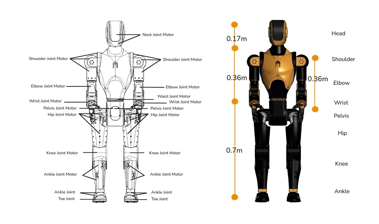
The ankle is where the design gets counterintuitive. 36 Nm looks light for a joint stabilizing the full body weight, but Asimov's ankle is not a serial joint. It is a parallel RSU mechanism: two motors drive pitch and roll through a shared linkage, so the load is distributed and serial-joint intuition does not apply.

That distinction matters far beyond the mechanical design. It propagates into simulation, into control, and into deployment. When you train a locomotion policy in simulation, the ankle is often modeled as directly actuated for simplicity; on hardware it is not. Deploying from sim to real therefore requires a kinematic remapping. Miss it, and the policy breaks at the joint level before it ever walks. The legs have 12 actuated joints, six per side, with no toe joint: push-off and forward balance recovery are handled entirely at the ankle, which is part of why the parallel ankle mechanism carries so much of the leg design.

Fabrication: what you can print and what you can't

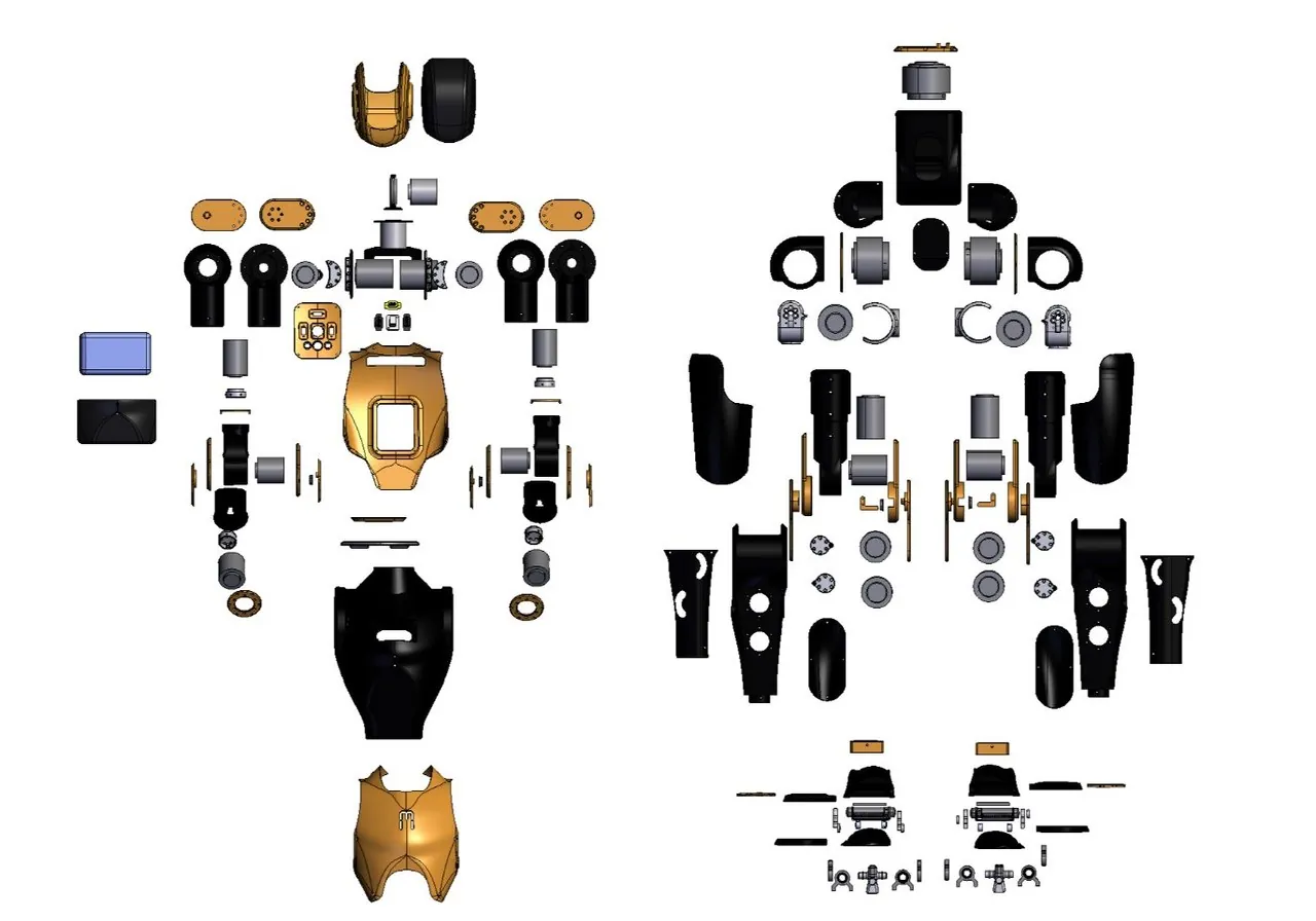
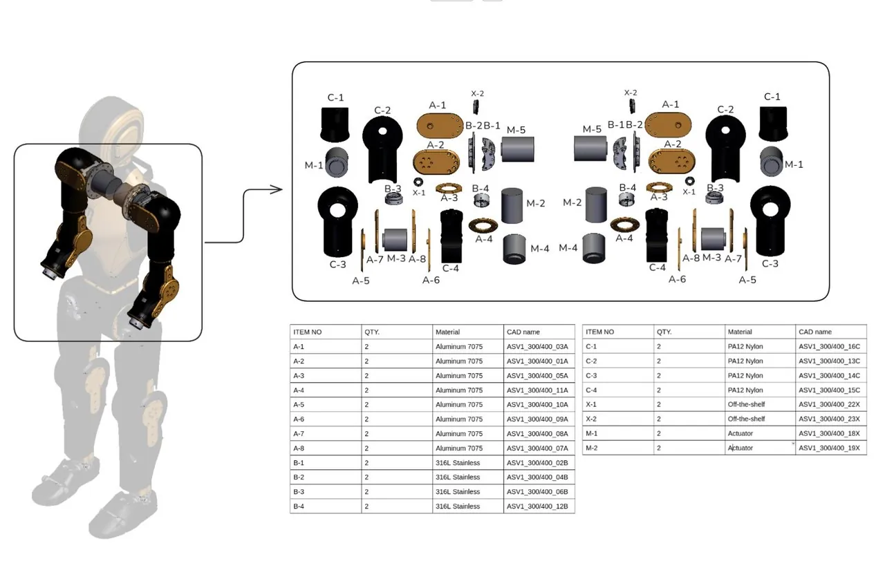
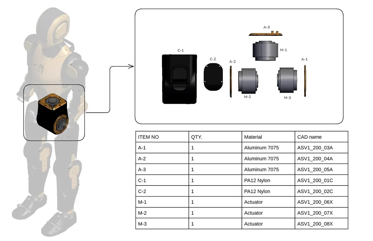
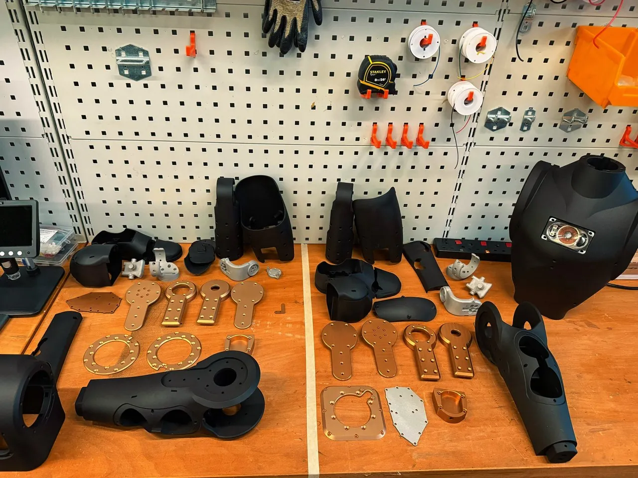
Every part follows a naming convention that tells you exactly how it should be made. The letter in the part name encodes the manufacturing method and material family.

Code	Process	Material	Typical use
A	CNC machining	Aluminum 7075	Load-bearing structure, e.g. hip pitch brackets
B	SLM metal printing	316L stainless steel	High-stress small parts
C	SLS / MJF printing	PA12 nylon	Cable routing brackets, covers, non-load-bearing structure
X	Off-the-shelf	—	Purchased components (actuators, fasteners, electronics)

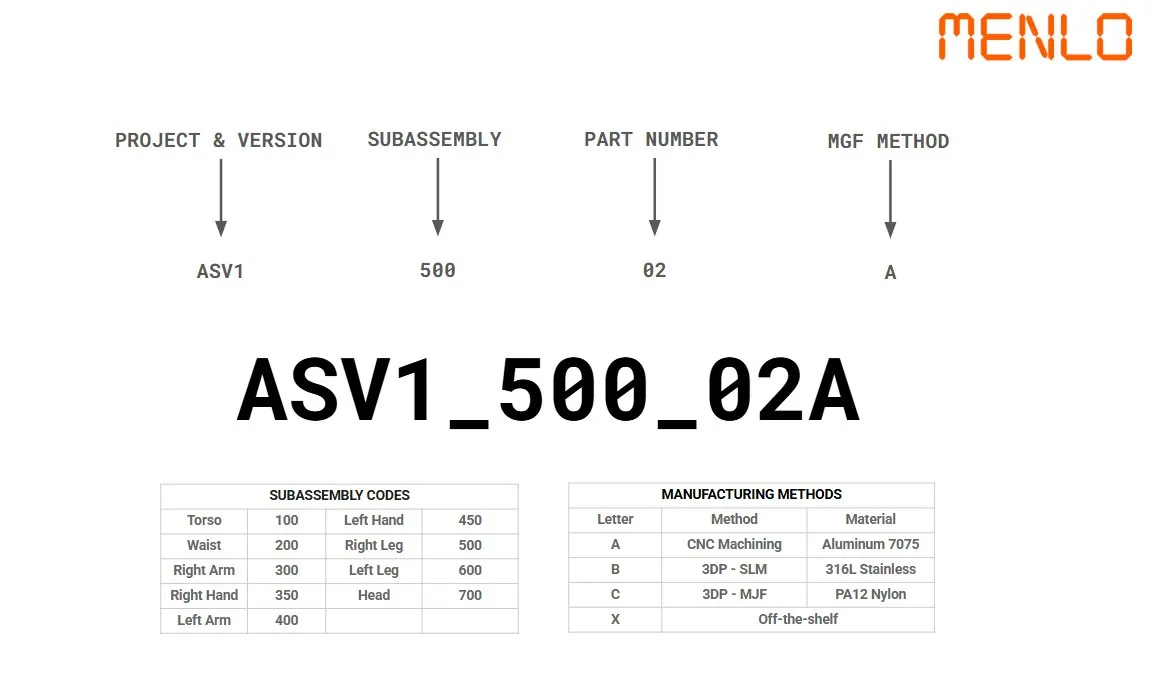
FDM printing will not work for structural components, and this is not a preference: it is a tolerance and strength problem. A hip pitch bracket machined from aluminum 7075 handles the repeated dynamic loading of a 35 kg robot in motion; the same bracket printed in PLA on a desktop printer cannot. It flexes under load, introduces play into the joint, and corrupts the mechanical assumptions the control stack was built on. Bad geometry at the bracket level propagates into bad contact geometry at the foot level, which propagates into bad training data, which produces a policy that cannot transfer. The failure chain starts at fabrication.

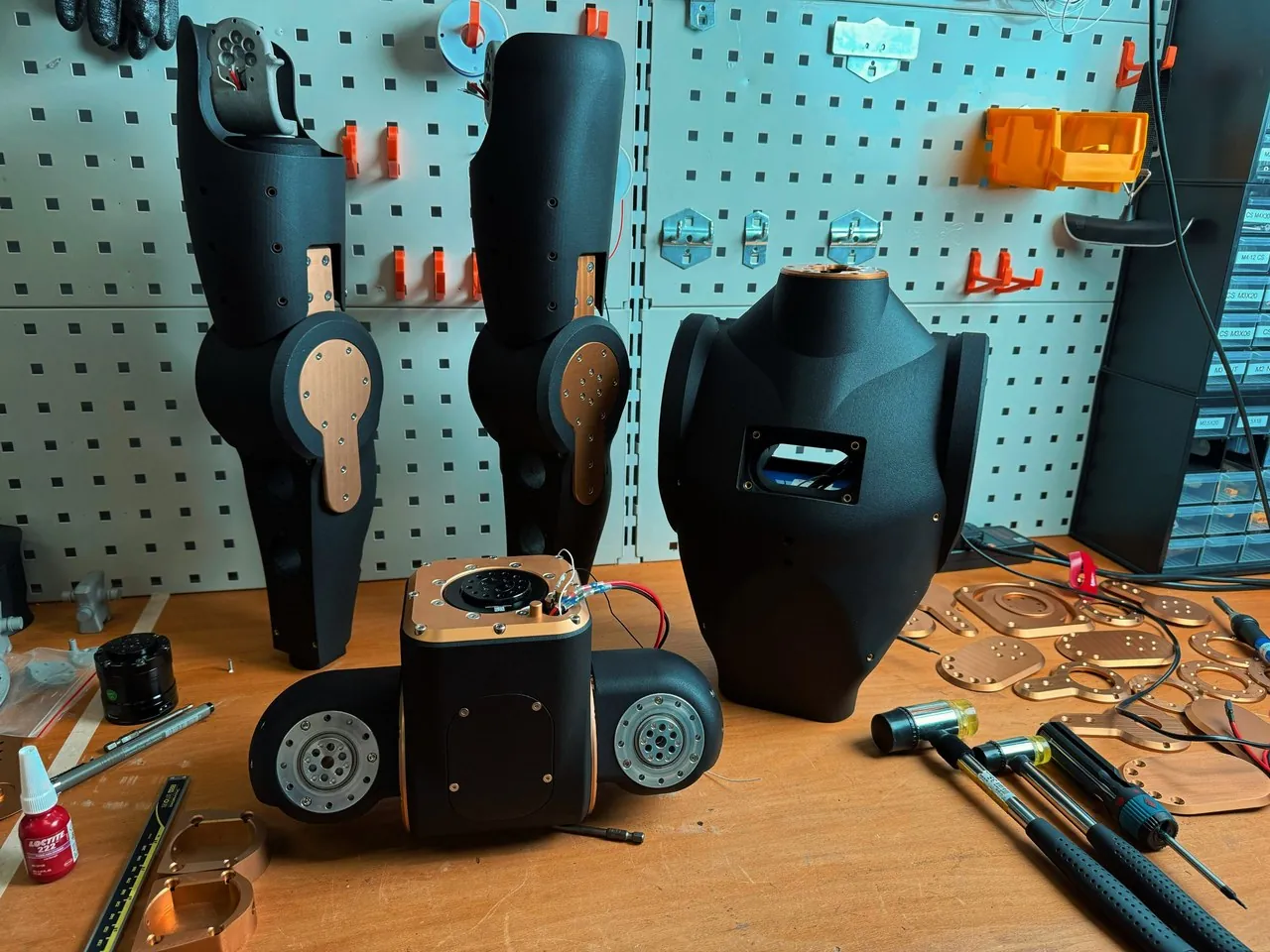
PA12 nylon printed via SLS or MJF is different: it works for cable routing brackets, covers, and non-load-bearing structure because those parts are not in the mechanical load path. The fabrication code tells you which category each part falls into. Follow it. If you are self-sourcing, the team recommends PCBWay or JLCMC for machined and printed parts, where lead times and quality are predictable; from the kit, parts arrive ready for assembly.

Electronics and wiring: CAN order is a control problem

The compute stack includes an edge board for high-level control, a motion control board for the internal bus, a network board, and a power distribution board. Motors communicate over CAN, and the IMU feeds into firmware over the same communication path.

Wiring is where most first-time builders spend unexpected time, and CAN bus ordering matters more than people expect. In early Asimov development, motor state requests were issued in sequence but responses could arrive in a different order. That is logically fine at the communication layer. It is not fine for control: the policy interprets stale and reordered state as a real physical deviation, applies corrective action too aggressively, and the resulting impulses excite oscillations across the legs. The robot shakes itself apart before it takes a step.

The fix is to make the real IO sampling path match what the training environment expects: sample actuators at the intended rate, wait for the expected packet order, and do not let communication-layer flexibility create timing ambiguity at the control layer. This is the kind of problem you only understand by building and wiring the robot yourself.

Simulation and the control problem

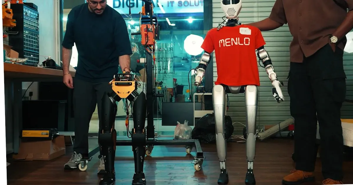
Walking is not a mechanical problem; it is a data problem. The locomotion policy is a neural network trained in simulation with reinforcement learning, and the central question is not how sophisticated the network is. It is whether the policy sees the same type, timing, and quality of data in simulation that it will see on hardware. Most sim-to-real failures are not caused by physics mismatches. They are caused by timing skew, stale observations, bus jitter, or control signals computed differently in simulation and on hardware. Get the physics right and the timing wrong, and the policy still breaks.

Asimov is past this: locomotion policies trained in simulation run on the robot with no fine-tuning and no on-robot iteration. The rates are separate by design.

Loop	Rate	Notes
Physics	200 Hz	Simulation step
Observation and IO	200 Hz	Joint groups polled in real CAN order; oldest group carries 0–2 steps of delay
Policy execution	50 Hz	The actor is never trained on perfectly fresh simulator state

The policy is deliberately not trained on perfectly fresh simulator state. It is trained on data that already reflects the timing artifacts of the control loop, because that is what the real robot produces. Joint observations are grouped to reflect the real CAN polling order: different joints arrive with different freshness, the oldest group with 0 to 2 steps of delay, the freshest with none. This staggered structure is not a simulation artifact; it is a deliberate model of what hardware does.

flowchart LR
    subgraph sim ["Simulation (training)"]
        phys["Physics\n200 Hz"] --> obs["Observations and IO\n200 Hz\njoint groups in CAN polling order\n0-2 step stagger"]
        obs --> actor["Actor MLP\n50 Hz\n45-dim observation"]
        obs --> critic["Critic (training only)\n+ ground-truth base velocity\nfoot height, air time,\ncontact state and forces"]
    end
    subgraph hw ["Robot (deployment)"]
        can["CAN bus\nmotors + IMU"] --> io["IO sampling\n200 Hz, fixed packet order"]
        io --> actorhw["Actor MLP\n50 Hz\njoint targets to motors"]
    end
    actor -- "same weights, zero fine-tuning" --> actorhw

The oscillation problem, and what it teaches

Early in development the robot oscillated violently on startup. The instinct is to add damping, retune rewards, or adjust hardware; none of those fixed it. The actual cause was two problems interacting.

First, the simulation PD gains produced an underdamped system. Low-level tracking on the robot is a standard proportional-derivative law,

$$\tau = K_p\,(q_{\mathrm{des}} - q) + K_d\,(\dot{q}_{\mathrm{des}} - \dot{q})$$

and the policy is just an MLP whose job is to model a function from the data it sees. Trained on underdamped simulation data, it learns underdamped control behavior and carries that onto real hardware. On hardware the gains are fine, but the policy's learned behavior overshoots; each overshoot triggers a larger correction, and sustained oscillation follows. Second, CAN packet ordering caused the policy to correct against state that no longer reflected reality, amplifying the oscillation on every cycle. Both had to be fixed together: fixing the gains alone did not work while the policy consumed misordered state, and fixing CAN ordering alone did not work while the controller was underdamped.

The lesson is not just "tune your gains carefully." It is that simulation and hardware must produce the same class of data. If the data domains diverge, the policy learns behavior that cannot transfer, regardless of whether individual parameter values look physically reasonable. You do not learn this from a paper; you learn it by building the robot, wiring it, watching it shake, and working backward through the control stack to find the cause.

Training the locomotion policy

The actor network observes 45 dimensions: IMU angular velocity, projected gravity, commanded velocities, joint positions grouped by CAN timing, joint velocities grouped by CAN timing, and previous actions. Formally,

$$o_t = \big[\ \omega_t,\ \tilde{g}_t,\ v^{\mathrm{cmd}}_t,\ \{q^{(k)}_{t-\Delta_k}\}_k,\ \{\dot{q}^{(k)}_{t-\Delta_k}\}_k,\ a_{t-1}\ \big], \qquad \Delta_k \in \{0, 1, 2\}$$

where each group $k$ of joints arrives with the staleness imposed by the CAN polling order. Ground-truth base linear velocity is intentionally excluded, because the real robot does not measure it: training with unavailable information produces brittle policies that break at deployment.

This is worth pausing on. Most locomotion baselines feed ground-truth base velocity into the policy because it makes training easier and faster: the policy converges quicker and the numbers look better. But at deployment that signal disappears. The robot has an IMU and encoder-derived joint state; it does not have a ground-truth velocity sensor. A policy trained on unavailable information learns to depend on it, and dependence on unavailable information is just a delayed failure.

The critic gets more. During training it receives everything the actor sees plus ground-truth base velocity, foot height, foot air time, foot contact state, and contact forces:

$$s_t = \big[\ o_t,\ v^{\mathrm{base}}_t,\ h^{\mathrm{foot}}_t,\ T^{\mathrm{air}}_t,\ c_t,\ F^{\mathrm{c}}_t \big]$$

Signal	Actor (deploys)	Critic (training only)
IMU angular velocity, projected gravity	Yes	Yes
Commanded velocities	Yes	Yes
Joint positions / velocities, CAN-grouped with 0–2 step stagger	Yes	Yes
Previous actions	Yes	Yes
Ground-truth base linear velocity	No	Yes
Foot height, air time, contact state, contact forces	No	Yes

This asymmetry between actor and critic is one of the more elegant parts of the design. The critic is a training-only component and never runs on the real robot, so it can receive simulator-only signals that help it learn better value estimates. The actor is the component that deploys, so it is restricted to signals that exist on hardware. The result is a policy trained with rich information but deployed with only what the robot can measure: the critic does the heavy lifting during training so the actor does not have to cheat at deployment.

There is no gait clock. Asimov's kinematics are specific to its hardware: the ankle range is limited by the parallel mechanism, and a hand-imposed gait phase borrowed from a different robot's geometry would constrain the policy unnecessarily. The policy discovers a gait that fits this hardware instead.

The reward set is compact: velocity tracking, orientation penalty, air-time reward, action smoothness, torque efficiency, posture shaping, stability penalties, and contact force limits. Reward design was not the main bottleneck. The policy became deployable only after the actuator model, timing model, and observation interface were made accurate; reward tuning on top of bad system identification produces nothing useful.

What you get at the end

With the final stack, Asimov walks forward, backward, and laterally, and recovers balance under external pushes; the same underlying policy handles all of these cases. Data collection works from camera, audio, IMU, and motor joint states. Basic walking works through teleoperation. Custom AI agents can be embedded via the cloud API, and a digital twin is available for simulation work before touching hardware.

The honest constraints of a v1 design: manipulation is out of scope for now (grippers arrive in a few months, and manipulation and locomanipulation follow on the same hardware), advanced locomotion like dancing is out of scope, and onboard training is out of scope. These are version-one boundaries, not permanent limitations.

Why build it yourself

The team reports spending over $100,000 learning humanoid robotics from the ground up so others do not have to start from zero: the BOM, CAD files, and simulation environment are public, and the baseline walking policy is open source, so you can read it, retrain it, or replace it.

When you build Asimov yourself, you understand why the ankle uses a parallel mechanism. You understand why CAN ordering matters for control. You understand why ground-truth base velocity cannot be an actor input. You understand the difference between a pristine simulator and one that models real timing. You cannot get that understanding from a YouTube video; you get it by assembling the robot, wiring the motors, running the policy, watching it fail, and fixing it. Most people who want to build a humanoid robot will read this and wait for more docs, a more polished kit, a better time. That time does not come. The builders who understand humanoid robotics are the ones who started before it was easy.

---

Source: this post is a full adaptation of the X article "How to build a humanoid robot at home" by Asimov (Menlo Research), published 2026-04-11. Reference material: menlo.ai/asimov-1, assembly manual docs.menlo.ai/asimov/1, kit page asimov.inc/diy-kit. All images and videos are by Asimov / Menlo Research.