DeFM: Learning Foundation Representations from Depth for Robotics

Authors: Manthan Patel, Jonas Frey, Mayank Mittal, Fan Yang, Alexander Hansson, Amir Bar, Cesar Cadena, and Marco Hutter. The work comes from the Robotic Systems Lab at ETH Zurich, with collaborators at UC Berkeley, NVIDIA, and Imperial College London. Paper: arXiv:2601.18923. Project: de-fm.github.io. Code: leggedrobotics/defm. Weights: Hugging Face.

The paper takes the DINOv2 recipe out of RGB. Instead of learning from color and texture, DeFM uses 60.4M depth images to train a ViT-L/14 teacher, then distills it into CNN and ViT students between 3.01M and 303.7M parameters. The evaluation reaches classification, segmentation, navigation, dexterous manipulation, and quadrupedal ladder climbing.

One-sentence summary

DeFM shows that depth can support transferable geometric, semantic, and affordance features, provided the model sees a mixed depth corpus and an input representation that keeps both relative structure and metric scale.

Why a new RGB encoder is not enough

Freezing a visual backbone and training only a control head is now standard in robot learning. RGB foundation models supply strong features, but simulated RGB rarely spans real lighting, material, and texture variation. Policies that exploit color cues can therefore fail when a simulated scene meets a real camera.

Depth behaves differently. A depth image records physical distance along the camera Z axis, usually from structured light, stereo infrared, solid-state LiDAR, or neural depth. Geometry is invariant to many appearance changes, and fast high-fidelity depth simulation makes the modality attractive for sim-to-real training.

Yet depth has lacked a general-purpose encoder. Most systems either reinterpret RGB checkpoints on depth images or train a task-specific CNN from scratch. The first route treats depth as three intensity channels and can lose metric information; the second route learns a representation tied to one environment and one sensor.

The authors frame the gap sharply: depth contains object size, free space, and physical affordances, but is often consumed as raw pixels. Their question is whether one encoder can serve manipulation centimeters away and navigation tens of meters away.

DeFM is their answer. It is not a task policy. It is a representation that can be frozen for classification and segmentation, or plugged into reinforcement-learning policies for navigation, manipulation, and locomotion. All pretrained variants are released.

A mixed corpus of 60.4M depth images

Curating depth data is not simply a matter of collecting more images. Real captures carry sensor noise, synthetic metric depth is clean but domain-narrow, and monocular-depth estimates scale well but lack absolute meters. DeFM deliberately combines all three sources.

The corpus contains 60.4M images from 18 datasets: 25.0M MDE-derived samples, 22.4M real captures, and 13.0M synthetic images. MDE samples include ImageNet-21k and SA-1B converted through Depth Anything V2. Real sources include Taskonomy, HM3D, ARKitScenes, ScanNet, GraspNet-1B, DROID, and DrivingStereo. Synthetic sources include Replica, Hypersim, TartanGround, TartanAir, and SHIFT.

Source	Samples	Role
MDE-derived depth	25.0M	Object diversity and relative geometry
Real depth	22.4M	Sensor noise, missing data, deployment realism
Synthetic depth	13.0M	Clean metric scale and environment diversity
Total	60.4M	18 datasets, from tabletop objects to outdoor navigation

The mixture is complementary rather than incidental. MDE gives relative structure without calibrated meters; synthetic data gives exact scale without real noise; real captures give deployment-like artifacts but limited coverage. The ablation section later shows that any single source is weakest on at least one segmentation benchmark.

Three-channel log-depth normalization

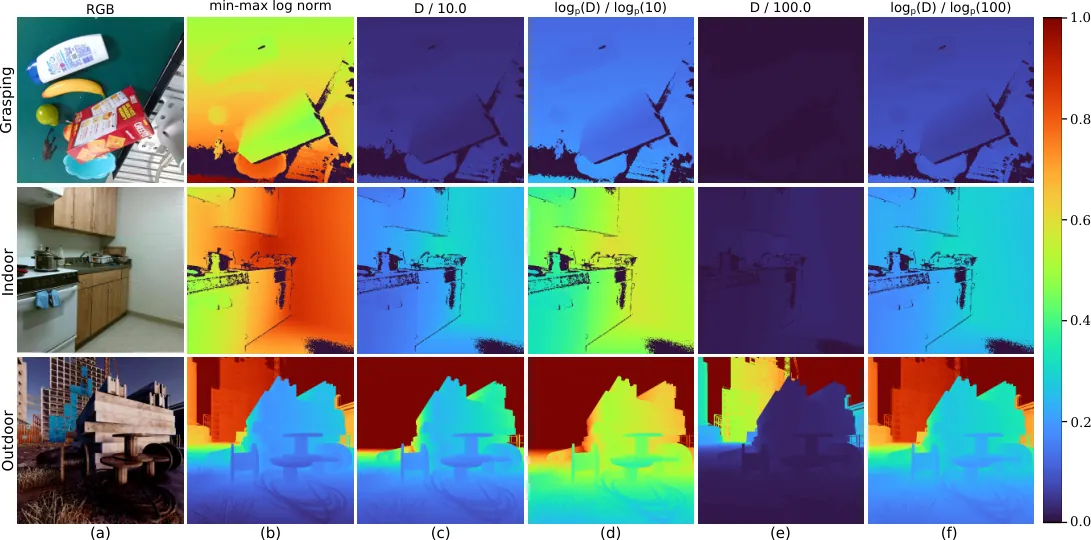
Depth ranges from millimeters to hundreds of meters. Linear normalization to 100 meters suppresses near-field variation, while purely local normalization loses the distinction between three meters and thirty meters. DeFM therefore uses three complementary logarithmic channels.

The paper defines:

$$\log_p(D)=\log(1+D)$$

The first channel is normalized by the minimum and maximum of the current image:

$$C_1=\frac{\log_p(D)-\log_p(D_{\min})}{\log_p(D_{\max})-\log_p(D_{\min})}$$

The second channel is a mid-range metric channel, nominally normalized by ten meters:

$$C_2=\frac{\log_p(D)}{\log_p(10)}$$

The third channel targets far-field navigation:

$$C_3=\frac{\log_p(D)}{\log_p(100)}$$

The model input stacks all three:

$$X_{\text{in}}=[C_1,C_2,C_3]$$

The released code adds an important compatibility note. In defm/utils/utils.py::convert_to_3channel_metric, the mid-range maximum is 9.0 rather than 10.0. The comment states that pretraining actually used $\log(10)$, while a direct implementation would use $\log1p(10)$; setting the maximum to 9.0 gives $\log1p(9)\approx\log(10)$:

def convert_to_3channel_metric(metric_depth, max_depth_c1=100.0, max_depth_c2=9.0):
    metric_depth = np.nan_to_num(metric_depth, nan=0.0, posinf=0.0, neginf=0.0)
    metric_depth = np.clip(metric_depth, 0, max_depth_c1)
    log_depth = np.log1p(metric_depth)
    c1 = log_depth / np.log1p(max_depth_c1)
    c2 = np.clip(log_depth / np.log1p(max_depth_c2), 0, 1)
    min_log, max_log = np.log1p(metric_depth.min()), np.log1p(metric_depth.max())
    c3 = (log_depth - min_log) / (max_log - min_log) if max_log > min_log else np.zeros_like(log_depth)
    return np.stack([c1, c2, c3], axis=-1)

For uncalibrated MDE images, $C_2$ and $C_3$ remain monotonic pseudo-scales and do not carry physical meters; $C_1$ stays valid because it is scale-invariant. The design therefore teaches the encoder to use metric priors where available and relative geometry where calibration is absent.

Self-distillation adapted to depth

The teacher is a ViT-L/14 with about 304M parameters. DeFM uses the DINOv2 FSDP implementation, two global crops at $224^2$, and eight local crops at $98^2$. The teacher receives complete global crops; the student receives local crops and masked global crops.

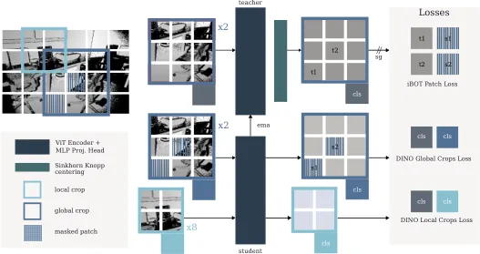
The global-crop loss aligns masked student views with unmasked teacher views:

$$\mathcal{L}_{\text{Global}}=\sum_{i=1}^{G}\sum_{j=1,j\neq i}^{G}\mathcal{L}_{\text{DINO}}(f_s(x'_{gi}),f_t(x_{gj}))$$

The local-crop loss teaches part-to-whole consistency:

$$\mathcal{L}_{\text{Local}}=\sum_{g=1}^{G}\sum_{l=1}^{L}\mathcal{L}_{\text{DINO}}(f_s(x_l),f_t(x_g))$$

The iBOT loss operates on masked patch tokens, where $p_{ti}$ is the teacher target and $p_{si}$ is the student prediction:

$$\mathcal{L}_{\text{iBOT}}=-\sum_{i\in\text{masked}}p_{ti}\log p_{si}$$

The total objective adds a KoLeo regularizer:

$$\mathcal{L}_{\text{total}}=\mathcal{L}_{\text{Global}}+\mathcal{L}_{\text{Local}}+\mathcal{L}_{\text{iBOT}}+\alpha\mathcal{L}_{\text{KoLeo}}$$

with $\alpha=0.1$. DINO and iBOT use separate projection heads and 131,072 prototypes. iBOT masks with probability 0.5 and mask ratios sampled uniformly from $[0.1,0.5]$. Teacher temperature rises from 0.04 to 0.07, and teacher momentum rises from 0.994 to 1.0.

Training follows the DINOv2 recipe rather than inventing a new optimizer schedule: AdamW, peak learning rate $3.5\times10^{-4}$, 100k warmup iterations, weight decay from 0.04 to 0.2, gradient clipping at 3.0, 625k iterations, batch size 3072, 96 GH200 GPUs, and float16 mixed precision.

The depth-specific changes are data, input, and augmentation. RGB color jitter, grayscale conversion, and solarization are removed. They are replaced with intensity jitter, Gaussian noise, and shared pixel dropout; the last operation simulates missing sensor depth so holes are not treated as a texture class.

flowchart TB
    D[Raw depth image] --> N[Three-channel log normalization]
    N --> C[Global and local crops]
    C --> T[Momentum ViT-L teacher]
    C --> M[Masking]
    M --> S[ViT-L student]
    T --> Q[Teacher targets]
    S --> L[DINO local loss]
    S --> L2[DINO global loss]
    S --> L3[iBOT patch loss]
    S --> L4[KoLeo regularizer]
    Q --> L
    Q --> L2
    Q --> L3
    L --> TOT[Total loss]
    L2 --> TOT
    L3 --> TOT
    L4 --> TOT

The source layout mirrors this flow: defm/models/vision_transformer.py implements the ViT and intermediate-layer API, defm/layers/dino_head.py contains the projection head, and defm/utils/utils.py::preprocess_depth_image converts arbitrary depth maps into patch-aligned tensors.

Distilling a ViT teacher into deployable CNNs

Downstream RL often benefits from large batches, while deployment requires low memory and latency. DeFM-L/14 is therefore frozen and distilled into ViT-S, ResNet, RegNet, and EfficientNet students. Distillation runs for 200k iterations on 64 GH200 GPUs with batch size 2048 and learning rate $1\times10^{-3}$.

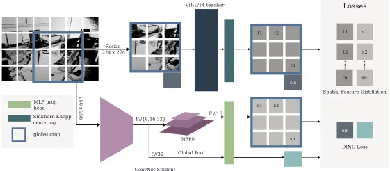
The main architectural issue is spatiality. Global average pooling can match a class token, but it discards the spatial layout that the ViT teacher retains in patch tokens. The authors add a BiFPN over CNN features at $F/8$, $F/16$, and $F/32$, fuse them top-down and bottom-up, and output dense maps at the same resolutions.

class BiFPNLayer(nn.Module):
    def forward(self, feats):
        td_feats[-1] = feats[-1]
        for i in range(self.n_levels - 2, -1, -1):
            up = F.interpolate(td_feats[i + 1], size=feats[i].shape[-2:], mode="nearest")
            td_feats[i] = self.fuse_topdown[i]([feats[i], up])
        for i in range(1, self.n_levels):
            down = F.max_pool2d(out_feats[i - 1], kernel_size=2, stride=2)
            out_feats[i] = self.fuse_bottomup[i - 1]([td_feats[i], down])
        return [conv(f) for conv, f in zip(self.convs, out_feats)]

The pooled CNN feature matches the teacher class token. The BiFPN output at $F'/16$ matches the teacher patch tokens. CNN inputs are $256\times256$, producing a $16\times16$ spatial map that aligns with the ViT-L/14 teacher on $224\times224$, where $224/14\approx16$. In defm/model_factory.py::create_defm_model, CNN backbones are constructed without torchvision ImageNet weights, preventing unrelated RGB priors from leaking into the depth student.

This is more than model compression. The student keeps two useful outputs: a global embedding and spatial features. The ablation makes the latter essential. Without a feature pyramid, ResNet-18 reaches only 14.81 mIoU on ScanNet; with BiFPN, it reaches 60.24.

Perception transfer: classification and segmentation

The authors introduce ImageNet-1k-Depth by converting RGB images with a monocular-depth model and running the DINOv2 linear-probe and KNN protocols. Because the classes and evaluation split follow the original object benchmark, this test measures whether the depth encoder has learned a linearly separable semantic space.

Model	Top-1 KNN	Top-5 KNN	Linear
ViT-L/14 DINOv2	60.28	80.75	68.26
ViT-L/16 C-RADIOv3	55.23	76.96	63.92
ViT-L/16 DINOv3	64.07	83.48	69.55
ViT-L/14 DeFM	63.46	84.79	71.72
ViT-S/14 DINOv2	47.66	69.11	55.06
ViT-S/16 DINOv3	49.50	70.93	50.86
ViT-S/14 DeFM	55.27	78.06	61.54

DeFM-L is best on Top-5 KNN and linear probing, and only 0.61 points behind DINOv3 on Top-1 KNN. The small-model result is more consequential: DeFM-S improves its size class by up to about 10 points, showing that depth-native pretraining matters even at modest capacity.

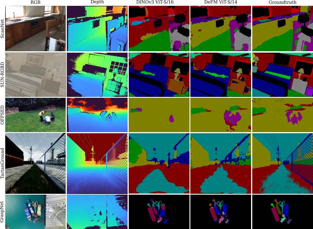
Segmentation uses frozen last-block patch tokens and a linear classifier, followed by bilinear upsampling. Five datasets test indoor rooms, outdoor infrastructure, off-road terrain, and tabletop grasping, so the probe also measures sensor and domain transfer.

Model	ScanNet	SUN-RGBD	OFFSED	TartanGround	GraspNet-1B
ViT-L/14 DINOv2	29.91	32.71	53.98	65.88	24.12
ViT-L/16 DINOv3	34.86	39.23	54.32	68.61	25.52
ViT-L/14 DAv2	29.91	32.68	55.87	67.25	25.43
ViT-L/14 DeFM	38.26	36.88	57.15	73.22	27.57
ViT-S/14 DeFM	33.79	33.27	58.10	70.82	20.53
ResNet-50 DeFM	35.34	32.19	52.55	70.89	31.95
ResNet-18 DeFM	28.01	25.97	46.87	65.49	23.27
PTv3-L Concerto	21.52	16.18	32.25	58.35	4.44
RE-PTv3 Utonia	23.06	20.70	30.36	59.79	4.34

DeFM-L is best on four of five datasets. DeFM-S shows a wider gap: on ScanNet it is 7.48 points above DINOv3-S and 14.23 points above Theia-S. Point-cloud foundation models underperform because unprojected single-view depth is a domain shift from their dense room scans, isolated objects, or LiDAR scenes.

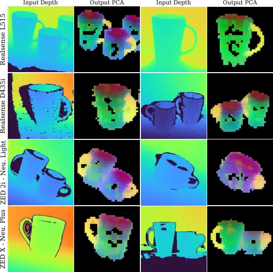
PCA visualization supports this interpretation. Across four depth sensors, handles and rims of different cups form stable clusters; drawer and cabinet handles are similarly highlighted. A grasping policy does not need to know the object's color to locate an interaction site.

Ablations isolate the design choices

The authors use a smaller ViT-S and 125k training steps so that design changes are not hidden by a long large-scale run. They ablate input normalization, data composition, and CNN distillation architecture, all evaluated with segmentation mIoU.

Variant	ScanNet	SUN-RGBD	OFFSED	TartanGround	GraspNet-1B
Relative log channel $C_1$ only	20.83	17.81	50.01	65.39	16.68
Far-range metric $C_3$ only	24.23	20.93	51.63	65.76	15.38
Three channels $[C_1,C_2,C_3]$	24.43	20.76	52.06	67.11	17.07
Real data only	27.80	22.62	49.20	65.01	15.06
Synthetic data only	21.75	18.66	50.23	67.14	15.31
MDE data only	22.74	18.93	49.78	65.87	14.12
Full mixture	24.43	20.76	52.06	67.11	17.07
ResNet-18 without FPN	14.81	12.96	40.50	57.75	18.30
ResNet-18 with standard FPN	17.18	15.46	45.81	58.93	16.88
ResNet-18 with BiFPN	17.13	16.35	42.39	60.24	19.32

The three-channel input wins four of five comparisons and loses only marginally to $C_3$ on SUN-RGBD. The far-range channel is strong overall but weak on GraspNet-1B, confirming that excessive compression hurts close-range tabletop geometry. The joint representation lets different probes exploit different priors.

Data composition tells a similar story. Real-only is best on ScanNet, synthetic-only is best on TartanGround, and MDE-only is weak on several benchmarks. The full mixture has the best average and is never the worst variant. The authors are careful to call this a reduced-scale result, not a proof of the optimal full-scale ratio.

The BiFPN result is less one-sided but still informative. It improves TartanGround by 2.49 and GraspNet-1B by 1.02 over no FPN; a standard FPN wins on ScanNet and OFFSED. Thus BiFPN is the best overall choice, while the broader conclusion is that multi-scale spatial fusion is necessary for dense distillation.

Navigation across held-out environments

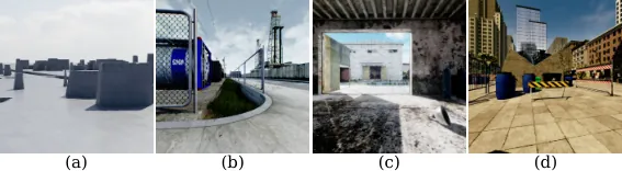
The navigation test uses Unitree B2W and embodiment-aware point-goal navigation. A frozen RegNetX-400MF with FPN supplies dense features, which cross-attend with proprioception before an SRU and MLP emit velocity commands. Training consists of mazes, pits, and stairs; held-out Gazebo environments are an industrial hangar, abandoned cable area, and modern city downtown.

Model	Training	Industrial Hangar	Abandoned Cable	Modern City Downtown
ImageNet	77.61	50.00	38.33	65.00
VAE	90.23	89.67	83.00	73.67
DINOv3	83.64	90.00	74.67	72.67
DeFM	90.31	92.67	84.33	79.00

VAE nearly matches DeFM during training, but DeFM is highest in all three held-out environments. Failure analysis shows fewer collisions for DeFM. The authors attribute this to recognizing thin out-of-distribution objects such as fences, traffic signs, and lamp posts. DINOv3 lags because depth is treated as intensity without multi-scale metric awareness.

Real deployments cover indoor, urban, park, and construction-site settings with goals from 5 to 100 meters. The policy handles pedestrians, scooters, barriers, furniture, and uneven terrain. The authors still report a limitation: wires, poles, and mesh structures can be missed at the low policy input resolution of $64\times40$, so higher resolution and more simulation diversity remain future work.

Manipulation and locomotion transfer

Dexterous grasping uses DexTRAH. A state-based teacher receives privileged object state and one-hot identity; the student receives depth images and feeds ResNet-18 features with proprioception into LSTM and MLP heads. Training uses eight L40S GPUs, 256 environments each, and depth augmentation with speckles, Gaussian noise, pixel dropout, and stick noise.

Pretraining	Frozen, training noise	Frozen, Kinect noise	Fine-tuned, training noise	Fine-tuned, Kinect noise
Scratch	—	—	0.7774	0.7247
ImageNet	0.6576	0.0043	0.7950	0.7366
VAE	0.6894	0.0219	0.8105	0.0379
DINOv3	0.6532	0.2075	0.8243	0.7837
DeFM	0.8089	0.4860	0.8936	0.8763

With frozen weights, DeFM exceeds the scratch student by 0.0315 and ImageNet by 0.1513 under training noise. Under the Kinect noise model, DeFM falls to 0.4860, while ImageNet and VAE collapse. After fine-tuning, DeFM reaches 0.8936 and 0.8763, so the representation supports both frozen use and task-specific adaptation.

Ladder climbing uses ANYmal. A CNN encoder, proprioception, and RNN form the student, trained with teacher-student distillation in IsaacGym using 1,024 environments, 120 collected steps per batch, and 10,000 epochs. Evaluation sweeps rung radii from 15 to 45 millimeters and ladder angles from 70 to 90 degrees.

CNN-Scratch	ImageNet	VAE	DINOv3	DeFM
90.45	89.29	89.75	89.59	90.14

DeFM is the best frozen model but remains 0.31 points behind the scratch CNN. The paper does not oversell this: pretraining does not beat every task-specific solution. The authors instead emphasize robustness to noisy real stereo depth and show PCA where ladder structure remains clustered under deployment noise.

Limitations and open problems

The authors acknowledge that curation is still primitive. Some sequential datasets are subsampled at 1–5 Hz while others are used in full, and deduplication has not been applied. They expect scaling data, model capacity, and iterations to improve capability once curation catches up.

Second, 25.0M MDE-derived images can import geometric artifacts, relative scale ambiguity, and RGB biases. Those maps are converted to a fixed pseudo-metric range, so their mid- and far-range channels do not carry true meters. Metric MDE or metric alignment is a natural extension.

Third, metric and lateral ambiguity remains, especially without camera intrinsics. The paper proposes learnable intrinsics, explicit metric tokens, or auxiliary depth reconstruction losses. Fourth, standard ViTs sometimes produce patch-level artifacts; register tokens may mitigate them. Fifth, solid-state LiDAR and LiDAR range images are not yet part of the model family.

There is also an engineering cost not discussed as a limitation: 60.4M images, 96 GH200 GPUs, and 625k iterations are a heavy investment. Distilled students address deployment, but most practitioners should use the released weights rather than reproduce the pretraining run.

Conclusion

DeFM is valuable because it closes the loop: a mixed depth corpus, metric-aware input, DINOv2/iBOT/KoLeo training, CNN and ViT distillation, perception and control evaluations, and public weights. The result is not just a depth autoencoder; it is a feature space with object parts, free space, and usable geometry.

For engineering use, the quickest path is to convert sensor depth with preprocess_depth_image, read class and patch tokens from get_intermediate_layers, or use the CNN dictionary containing global_backbone and dense_bifpn. DeFM does not eliminate task-specific encoders, but it supplies the general geometric and semantic prior so downstream policies start from a stronger visual representation.

A strong foundation model should point to graspable, traversable, and dangerous regions even when the input has no texture at all.