SiamJEPA: On the Role of Siamese Student Encoders in JEPA

Paper Information

Title: SiamJEPA: On the Role of Siamese Student Encoders in JEPA

Author: Makoto Yamada (Okinawa Institute of Science and Technology, OIST)

Paper: arXiv:2607.04044

Code: github.com/oist/SiamJEPA (public)

Published: July 2026 (v2: July 30, 2026)

One-Sentence Summary

SiamJEPA introduces Siamese student encoders into the JEPA framework, using KL regularization to enforce consistency between two masked views, achieving high-quality visual representations with fewer training epochs than pixel-reconstruction methods.

Background and Motivation

Self-supervised learning (SSL) has become a fundamental technique for learning transferable representations from large-scale unlabeled data in computer vision, natural language processing, and robotics. Unlike supervised learning, SSL extracts semantic information without labels, providing a universal feature basis for downstream tasks. In robotics, high-quality visual representations are essential for perception, manipulation, and navigation — from object recognition in grasping to scene understanding for mobile robots.

Joint embedding architectures form a major branch of SSL. Their core idea is to map different views of the same input into a shared latent space. SimCLR uses contrastive learning to pull positive pairs together and push negative pairs apart. BYOL and SimSiam demonstrated that negative samples are not strictly necessary, using stop-gradient operations and EMA teacher networks to prevent representation collapse. The DINO family extended this to Vision Transformers, achieving remarkable results through large-scale engineering.

Joint Embedding Predictive Architectures (JEPAs) represent the latest evolution of joint embedding methods. Instead of directly aligning latent representations, JEPAs learn to predict masked latent representations from visible context — operating in latent space rather than pixel space. I-JEPA and V-JEPA are representative works. The advantage of JEPA is that it skips pixel-level reconstruction and directly captures semantic information, potentially learning useful representations more efficiently. V-JEPA 2 has even extended this to world-model learning, demonstrating JEPA's potential for video understanding and predictive planning.

However, existing JEPA models (I-JEPA, V-JEPA) all employ a single student encoder. Meanwhile, the brain-inspired learning model PhiNet proposed Siamese student encoders, drawing inspiration from the biological circuitry of the hippocampus and neocortex — Siamese encoders correspond to the temporal predictive hypothesis, while the EMA mechanism corresponds to fast and slow learning in Complementary Learning Systems (CLS) theory. But what role Siamese encoders play within the JEPA framework has not been systematically investigated. This is the central question this paper addresses: What role do Siamese student encoders play in JEPAs?

Furthermore, masked Siamese methods such as SiamMAE, CropMAE, and RSP also use Siamese encoders, but they remain fundamentally reconstruction-based approaches targeting pixel or feature-level recovery. While they demonstrate strong performance on dense prediction tasks like segmentation and pose estimation, their effectiveness for learning general-purpose visual representations is less understood. SiamJEPA fills this gap by combining Siamese encoders with latent prediction objectives in a unified framework.

Preliminaries

JEPA Framework: Given a patchified input $\bm{X} \in \mathbb{R}^{m \times d_{\text{in}}}$ where $m$ is the number of patches, JEPA sends visible regions through a student encoder and the full image through an EMA teacher encoder. A predictor is then trained to forecast the teacher's latent representations of masked regions. Prediction occurs in latent space, without pixel reconstruction.

EMA Teacher Network: The teacher encoder $f_{\text{ema}}$ is not updated via gradients but through an exponential moving average of student parameters: $\theta_{\text{ema}} \leftarrow \alpha \cdot \theta_{\text{ema}} + (1-\alpha) \cdot \theta$. This mechanism, originating from BYOL and DINO, provides stable target representations and prevents training collapse.

Siamese Encoders: Two encoder networks with shared weights processing different views of the same input. In SiamJEPA, two Siamese student encoders receive different masks $M_1$ and $M_2$, producing two complementary representations whose consistency is enforced through regularization.

Probabilistic Predictor: SiamJEPA's predictor adopts a probabilistic framework from stochastic video generation and DreamerV2 — modeling latent representation uncertainty through KL divergence between a posterior $q(\bm{Z}|\text{both views})$ and a prior $p(\hat{\bm{Z}}|\text{single view})$, encouraging the encoder to capture information shared across views.

Method

Overall Architecture

The key modification in SiamJEPA is adding a second encoder to the student side of standard JEPA. While standard JEPA uses one student encoder for visible context and one predictor for target regions, SiamJEPA uses two weight-shared Siamese student encoders that process the same image with different masks $M_1$ and $M_2$, each with its own predictor to forecast the teacher's masked representations.

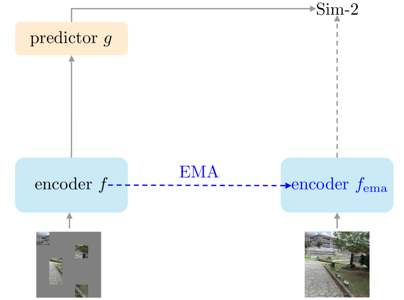
Figure 1a: Standard JEPA architecture. The student encoder processes visible context, and the predictor forecasts the teacher's latent representations of masked regions.

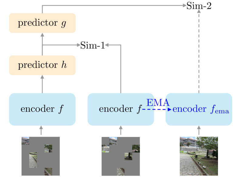
Figure 1b: SiamJEPA architecture (a.k.a. PhiNet architecture). Two Siamese student encoders process different masked views, with Sim-1 loss aligning their outputs.

Figure 1: JEPA and SiamJEPA architectures. Sim-1 is the loss function to align Siamese encoders. Dashed lines represent stop-gradient.

Siamese Student Encoders

Let $\bm{X} \in \mathbb{R}^{m \times d_{\text{in}}}$ denote the patchified input image with $m$ patches. The outputs of the two Siamese student encoders and the teacher encoder are:

$$\bm{H}^{(1)} = f(\text{Mask}(\bm{X}, M_1)), \quad \bm{H}^{(2)} = f(\text{Mask}(\bm{X}, M_2)), \quad \bm{Y} = f_{\text{ema}}(\bm{X})$$

where $\bm{H}^{(1)} \in \mathbb{R}^{N \times (m_1+1) \times d}$, $\bm{H}^{(2)} \in \mathbb{R}^{N \times (m_2+1) \times d}$, and $\bm{Y} \in \mathbb{R}^{N \times (m+1) \times d}$ are the output representations. $N$ is the batch size, $m_1 = |M_1|$ and $m_2 = |M_2|$ are the numbers of unmasked tokens, and $d$ is the embedding dimension. $f(\cdot)$ denotes the Siamese student encoder with shared weights, while $f_{\text{ema}}(\cdot)$ is the EMA teacher encoder. $\text{Mask}(\bm{X}, M)$ is the masking operator.

A critical design choice is that the two masking sets are disjoint: $M_1 \cap M_2 = \emptyset$. This non-overlapping masking strategy is crucial for preventing shortcut learning — if both encoders saw the same tokens, they could produce consistent outputs through simple copying rather than learning semantic representations.

The encoder outputs are further decomposed into CLS and patch tokens:

$$\bm{H}^{(1)} = [\bm{H}_{\text{cls}}^{(1)}; \bm{H}_{\text{patch}}^{(1)}], \quad \bm{H}^{(2)} = [\bm{H}_{\text{cls}}^{(2)}; \bm{H}_{\text{patch}}^{(2)}], \quad \bm{Y} = [\bm{Y}_{\text{cls}}; \bm{Y}_{\text{patch}}]$$

where $\bm{H}_{\text{cls}} \in \mathbb{R}^{N \times 1 \times d}$ is the CLS token representation and $\bm{H}_{\text{patch}} \in \mathbb{R}^{N \times m \times d}$ is the patch token representation.

Predictor Networks

SiamJEPA employs two predictors: a linear predictor $h(\cdot)$ and a Transformer predictor $g(\cdot)$.

The linear predictor $h$ aligns the global representations of the two Siamese student encoders:

$$h(\bm{H}) = \bm{H}\bm{W}$$

where $\bm{W} \in \mathbb{R}^{d \times d}$ is a linear transformation matrix that helps align the representation spaces of the two Siamese student encoders.

The Transformer predictor $g$ predicts the latent representations of masked regions. SiamJEPA adopts a probabilistic prediction framework, defining posterior and prior distributions:

$$\text{Posterior:} \quad \bm{Z}^{(1)} \sim q(\bm{Z}^{(1)} | h(\bm{H}_{\text{cls}}^{(1)}), \bm{H}_{\text{cls}}^{(2)})$$

$$\text{Prior:} \quad \hat{\bm{Z}}^{(1)} \sim p(\hat{\bm{Z}}^{(1)} | h(\bm{H}_{\text{cls}}^{(1)}))$$

The posterior incorporates information from both Siamese branches, while the prior is conditioned only on the first branch's representation. Symmetrically, swapping the branches yields $\bm{Z}^{(2)}$ and $\hat{\bm{Z}}^{(2)}$. The latent variable $\bm{Z}$ models the uncertainty of the latent representation given the available context. Both $q(\cdot)$ and $p(\cdot)$ are parameterized by two-layer neural networks, with a projector head using batch normalization applied before constructing the distributions.

The Transformer predictor outputs are:

$$\hat{\bm{Y}}^{(1)} = g(h(\bm{H}^{(1)}), \bm{Z}^{(1)}) \in \mathbb{R}^{N \times (m+1) \times d}$$

$$\hat{\bm{Y}}^{(2)} = g(h(\bm{H}^{(2)}), \bm{Z}^{(2)}) \in \mathbb{R}^{N \times (m+1) \times d}$$

Loss Functions

The total SiamJEPA loss combines two components: KL divergence between Siamese encoders (Sim-1) and MSE prediction loss against teacher representations (Sim-2).

Sim-1: KL Divergence Regularization. By constraining the KL divergence between posterior and prior, the two Siamese encoders are encouraged to produce consistent latent representations:

$$\text{KL}_{\text{sg}}^{(1)} = \text{KL}(q(\bm{Z} | [h(\bm{H}_{\text{cls}}^{(1)}), \bm{H}_{\text{cls}}^{(2)}]) \| \text{sg}(p(\bm{Z} | h(\bm{H}_{\text{cls}}^{(1)}))))$$

$$\text{KL}_{\text{sg}}^{(2)} = \text{KL}(q(\bm{Z} | [h(\bm{H}_{\text{cls}}^{(2)}), \bm{H}_{\text{cls}}^{(1)}]) \| \text{sg}(p(\bm{Z} | h(\bm{H}_{\text{cls}}^{(2)}))))$$

where $\text{sg}(\cdot)$ is the stop-gradient operator. This design requires the prior (inferred from a single view) to match the posterior (inferred from both views), encouraging the encoder to capture information shared across views while discarding view-specific variations.

Sim-2: MSE Prediction Loss. Measures the discrepancy between predicted and teacher representations for masked regions:

$$\text{MSE}^{(1)} = \frac{1}{|\bar{M}|} \|\text{Mask}(\bm{Y}_{\text{patch}}^{(1)} - \hat{\bm{Y}}_{\text{patch}}^{(1)}, \bar{M})\|_{\text{Frob}}^2$$

$$\text{MSE}^{(2)} = \frac{1}{|\bar{M}|} \|\text{Mask}(\bm{Y}_{\text{patch}}^{(2)} - \hat{\bm{Y}}_{\text{patch}}^{(2)}, \bar{M})\|_{\text{Frob}}^2$$

where $\|\cdot\|_{\text{Frob}}$ is the Frobenius norm and $\bar{M} = M \setminus (M_1 \cup M_2)$ is the complement of the union of both mask sets, with $M = \{1, 2, \ldots, m\}$ being the set of all patch indices. The prediction targets are regions in the teacher's output that are covered by neither $M_1$ nor $M_2$.

Total Loss:

$$\mathcal{L} = \frac{1}{2}(\text{MSE}^{(1)} + \text{MSE}^{(2)}) + \frac{\lambda_{\text{KL}}}{2}(\text{KL}_{\text{sg}}^{(1)} + \text{KL}_{\text{sg}}^{(2)})$$

The parameter $\lambda_{\text{KL}}$ controls the strength of Siamese encoder consistency. When $\lambda_{\text{KL}} = 0$, SiamJEPA reduces to a model similar to single-encoder JEPA. This unified formulation enables systematic investigation of the contribution of Siamese encoders.

graph LR
    A["Input Image X"] --> B["Mask M1"]
    A --> C["Mask M2"]
    A --> D["EMA Teacher f_ema"]
    B --> E["Student Encoder f
Branch 1"]
    C --> F["Student Encoder f
Branch 2"]
    D --> G["Teacher Repr Y"]
    E --> H["Linear Predictor h"]
    F --> H
    H --> I["Probabilistic Predictor
Posterior q / Prior p"]
    I --> J["KL Divergence
Sim-1 Regularization"]
    I --> K["Transformer Predictor g"]
    K --> L["MSE Loss
Sim-2 Prediction"]
    G --> L
    J --> M["Total Loss L"]
    L --> M

Figure 2: SiamJEPA data flow. The input image passes through three paths — two Siamese student encoders with different masks and one EMA teacher — jointly trained via KL regularization and MSE prediction loss.

Key Differences from Standard JEPA

The core distinction between SiamJEPA and standard I-JEPA is the dual-encoder design on the student side. I-JEPA uses one student encoder for visible context and one predictor for target regions; SiamJEPA uses two Siamese student encoders processing different masked views, with KL regularization enforcing their consistency. This means SiamJEPA not only learns to predict masked representations but also learns to produce consistent latent representations from different masked perspectives — constituting an additional inductive bias.

Another important difference is the predictor architecture. I-JEPA uses a relatively deep Transformer predictor, while SiamJEPA finds that a shallow predictor with only 1-2 layers suffices. This is advantageous for parameter efficiency. The paper suggests that shallow predictors combined with Siamese encoders may work because the Siamese architecture itself provides part of the predictor's capability.

Training Configuration

SiamJEPA uses ViT-Base as the backbone, pre-trained on ImageNet-1K. The effective batch size is 8192, predictor depth is 1, and the base learning rate is $1.5 \times 10^{-4}$. The EMA momentum follows a piecewise schedule: 0.99 for epochs 1-200, 0.999 for epochs 201-300, and 0.9999 for epochs 301-400. Mask ratios are selected from $\{0.7, 0.75, 0.8\}$. The implementation is built upon the official MAE codebase rather than I-JEPA's, providing a unified comparison framework for reconstruction-based and JEPA-based methods.

Figure 3: Pretraining and linear probing configurations. SiamJEPA uses a shallower predictor (depth 1 vs MAE's 8) and a larger effective batch size.

Experimental Results

Comparison with Other SSL Methods

On the ImageNet linear probing benchmark, SiamJEPA achieves 70.7% Top-1 accuracy after 400 training epochs, surpassing MAE's 61.9% at 400 epochs (and approaching MAE's 68.0% at 1600 epochs), while being comparable to CAE's 70.4% at 1600 epochs. This means SiamJEPA achieves higher accuracy with less than one-quarter of MAE's training epochs, demonstrating significant training efficiency advantages.

Method	Epochs	Top-1 Acc. (%)
MAE	400	61.9
MAE	1600	68.0
CAE	1600	70.4
I-JEPA	600	72.9
JEPA-like ($\lambda_{\text{KL}}=10^{-5}$)	400	68.9
SiamJEPA ($\lambda_{\text{KL}}=0.01$)	400	70.7

Table 1: ImageNet linear probing performance. SiamJEPA at 400 epochs surpasses MAE at 1600 epochs.

Compared to I-JEPA, SiamJEPA's final accuracy is lower (70.7% vs 72.9%), but the paper notes this comparison is not direct: I-JEPA was trained for 600 epochs with a different setup. SiamJEPA's goal is not to achieve SOTA but to validate the role of Siamese encoders in JEPA.

Regularization Effect of Siamese Encoders

Ablation experiments clearly show the impact of KL regularization weight $\lambda_{\text{KL}}$. Increasing from $\lambda_{\text{KL}} = 0.00001$ to $0.01$ or $0.03$ improves linear probing accuracy at all training stages. At epoch 101, $\lambda_{\text{KL}}=0.01$ reaches 63.72% while $\lambda_{\text{KL}}=0.00001$ only achieves 60.88% — meaning the consistency constraint produces significant gains early in training. The $\lambda_{\text{KL}}=0.01$ model at 200 epochs reaches the level that $\lambda_{\text{KL}}=0.00001$ achieves at 400 epochs, validating the convergence acceleration effect of Siamese encoders.

$\lambda_{\text{KL}}$	Weight Decay	Ep.51	Ep.101	Ep.201	Ep.301	Ep.400
0.00001	0.05	49.75	60.88	66.12	68.21	68.91
0.010	0.05	51.64	63.72	68.00	69.30	69.33
0.030	0.05	51.37	63.58	68.42	69.05	69.24
0.00001	0.1	48.85	58.99	57.68	62.55	62.54
0.010	0.1	48.83	63.44	67.84	69.57	70.15
0.030	0.1	47.47	62.63	67.97	69.82	70.17

Table 2: Ablation of KL regularization weight and weight decay. $\lambda_{\text{KL}}=0.01$ with weight decay=0.1 achieves the best final performance (70.15%).

Effect of Masking Strategy

The paper compares random masking and block masking. Block masking consistently outperforms random masking across all configurations, with a particularly large gap in early training — at epoch 51, block masking (ratio 0.75) achieves 51.64% while random masking only reaches 32.27%. However, as training progresses, random masking with a properly tuned ratio can also achieve decent performance (65.10%). This finding suggests that strong JEPA-style representations may be learnable without carefully designed masking schemes, which has positive implications for practical deployment.

Interestingly, at mask ratio 0.8, random masking (67.10%) actually outperforms block masking (66.79%), suggesting that the gap between strategies narrows at higher mask ratios. The effective mask ratio (regions not contributing gradients in either direction) is approximately 0.5 at mask ratio 0.75, meaning the model must predict representations for half the patches from the other half's information.

Effect of Representation Type

The paper compares CLS token, 10th-layer mean pooling, and 12th-layer (final) mean pooling for linear probing. The 10th-layer mean pooling performs best during early training, while 12th-layer mean pooling gradually catches up and sometimes surpasses it with sufficient training. This suggests that intermediate layers acquire linearly separable semantic representations earlier, while the final layer initially specializes in the pretraining objective before gradually learning more transferable representations. Mean pooling overall outperforms CLS token, indicating that useful semantic information is distributed across patch representations rather than concentrated in the CLS token.

Effect of EMA Scheduling

A larger EMA momentum (0.9999) leads to mode collapse, while a smaller momentum (0.999) continues to improve performance. Under $\lambda_{\text{KL}}=0.01$ and weight decay=0.1, EMA momentum 0.999 achieves 70.15% while 0.9999 collapses. The paper notes that the EMA schedule was empirically determined and there is room for improvement. This finding is consistent with experiences in BYOL and DINO — excessively large EMA momentum may cause the teacher to update too slowly, creating divergence from the student that is detrimental to the Siamese architecture's consistency constraint.

Limitations

Does not achieve SOTA performance (author-stated). SiamJEPA's goal is not to maximize benchmark scores but to validate the role of Siamese encoders. Compared to I-JEPA (72.9%), SiamJEPA (70.7%) has lower absolute accuracy, and the training setups differ, making direct comparison inappropriate. The authors acknowledge that performance could be further improved through more extensive hyperparameter optimization and longer training, but this is beyond the paper's scope.

Insufficient study of predictor depth (author-stated + our assessment). Due to computational constraints, the paper could not systematically explore the effect of predictor depth. While 1-2 layer shallow predictors work best empirically, the authors are uncertain whether this is an intrinsic property of SiamJEPA or specific to the current experimental setting. This question is critical for understanding the architecture's design principles but requires more computational resources.

Only validated on ImageNet (our assessment). All experiments are conducted on ImageNet-1K linear probing, without testing downstream tasks (e.g., detection, segmentation) or larger-scale datasets. The effectiveness of Siamese encoders on dense prediction tasks — particularly given the advantages of SiamMAE on pose estimation and segmentation — remains to be verified. Additionally, model scales beyond ViT-Base (e.g., ViT-Large or ViT-Huge) are not covered, leaving SiamJEPA's scalability unclear.

Unfair comparison with I-JEPA (our assessment). The implementation is based on the MAE codebase rather than the official I-JEPA implementation, resulting in different training dynamics. While this provides a unified comparison framework for reconstruction and JEPA methods, it also means the performance gap with I-JEPA may partly stem from implementation differences rather than methodological advantages.

Conclusion and Future Work

SiamJEPA provides the first systematic study of Siamese student encoders within the JEPA framework. The core finding is that Siamese encoders are not merely an architectural choice but constitute an important inductive bias for predictive representation learning. By enforcing consistency between two masked views through KL regularization, Siamese encoders act as an effective regularizer that constrains the representation space, improves separability, and accelerates early-stage convergence. Under limited training budgets, SiamJEPA consistently outperforms comparable single-encoder JEPA variants.

More broadly, SiamJEPA's significance lies in connecting two previously parallel research directions: the JEPA family (I-JEPA, V-JEPA) and brain-inspired learning (PhiNet). The paper demonstrates that PhiNet's Siamese architecture can be naturally incorporated into the JEPA framework with substantial performance gains. This unified perspective offers new insights for future JEPA model design.

The paper also reveals practical findings: random masking can be competitive with block masking when properly tuned, and shallow predictors suffice for good performance — these findings lower the implementation barrier for JEPA methods and facilitate broader adoption. For robotics, more efficient visual representation learning means better perception can be achieved with less labeled data and compute, which is practically valuable for deploying SSL models on resource-constrained robot platforms.

Future directions include: systematically studying the relationship between predictor depth and representation dynamics, validating SiamJEPA's scalability on larger models and datasets, exploring the role of Siamese encoders in video JEPA models like V-JEPA, and applying SiamJEPA to downstream tasks in robot perception and world-model learning.

Golden Quote

"Siamese student encoders are not merely an architectural choice but constitute an important inductive bias for predictive representation learning."