PAPER DEEP DIVE
Efficient-WAM: A 1B-Parameter World-Action Model with Low-Cost Future Imagination
World-Action Models (WAMs) have emerged as a promising paradigm for embodied control by coupling future visual prediction with action generation. However, many existing WAMs rely on photorealistic future prediction, which incurs high inference latency and makes real-time robot deployment difficult. We introduce Efficient-WAM, a World-Action Model motivated by the idea that a compact future branch can still support effective action generation, even at lower visual fidelity. Efficient-WAM improves inference efficiency via a compact video expert transferred from WAN-2.2-5B, token-sparse video latents, and asymmetric video-action denoising that allocates fewer sampling steps to video than to actions. Instead of prioritizing visual fidelity, Efficient-WAM treats future video prediction as a compact guidance signal for action generation. Experiments on RoboTwin 2.0 and real-world manipulation tasks show that Efficient-WAM maintains strong action performance despite visibly coarse future predictions. Our 1B-parameter model achieves 98 ms per action chunk during physical deployment, over 30x faster than the Motus baseline with comparable task success.
One-line summary
Efficient-WAM compresses the video branch of a World-Action Model along three axes at once: a 0.8B compact video expert sliced and distilled from WAN-2.2-5B, future frames downsampled to 192x160 so future tokens drop to one quarter, and training-free asymmetric denoising that updates video only in the first two of ten action iterations. The resulting 1B-parameter model runs at 98 ms per action chunk on real hardware with success comparable to the 8B Motus.
1. Background and Motivation
World-Action Models (WAMs) couple future visual prediction with action generation: given a current observation $o$, a language instruction $l$, and a robot state $s$, the model predicts future visual latents $\mathbf{z}^{v}$ together with an action chunk $a_{1:H}$. Because forecasting how the scene will evolve forces the policy to internalize physical dynamics and world priors, WAMs have become an attractive route in robot learning.
The cost of this route concentrates in the video branch. Most WAMs inherit the heavy design of video generators: large backbones, dense visual tokens, iterative denoising. Motus, for instance, needs 3215 ms per action chunk on an RTX 4090 (Table 2), while a 16-step chunk typically covers only a few hundred milliseconds of robot execution. High-fidelity future prediction therefore drags the control loop far below real time and blocks physical deployment.
Existing evidence suggests control tolerates lower video fidelity than intuition implies. VPP shows that action generation stays effective even when video denoising is reduced to a single step, and Fast-WAM shows that a WAM remains competitive when explicit future generation is skipped entirely at inference. Together they indicate that the video branch carries substantial headroom for reduction, and that the guidance function need not vanish when fidelity drops.
This paper turns that observation into a design question: can a streamlined video branch still supply useful guidance for action generation at visibly reduced fidelity? To make the question engineerable, the authors write video-side inference cost as a function of three controllable factors, the active video model size $\mathcal{M}_{v}$, the future token count $N_{\text{tok}}^{v}(r_{v})$ set by future resolution, and the video denoising budget $K_{v}$, and attach one mechanism to each: a compact video expert, low-resolution future latents, and asymmetric video-action denoising.
The division of labor with prior efficiency work is then clear. Early-exit and dynamic layer-skipping methods cut policy-backbone computation, and diffusion-policy distillation or single-step denoising accelerates action sampling; none of them touches the video-imagination bottleneck specific to WAMs. This paper isolates that bottleneck, measures each factor with dedicated ablations, and validates the combined design on real robots.
2. Preliminaries
Conditional flow matching. Both branches train with conditional flow matching: with clean target $\mathbf{x}_{0}$ (future latents or actions) and noise $\mathbf{x}_{1}\sim\mathcal{N}(0,I)$, the interpolation path is $\mathbf{x}_{t}=(1-t)\mathbf{x}_{0}+t\mathbf{x}_{1}$ with target velocity $\mathbf{u}_{t}=\mathbf{x}_{1}-\mathbf{x}_{0}$; the model regresses this velocity with mean squared error, and sampling integrates from $t=1$ to $t=0$. Video and action noise levels are sampled independently during joint training, which is precisely what allows the later asymmetric schedule to change inference without retraining.
Mixture-of-Transformers. The backbone is a MoT: the video stream and the action stream keep separate projections and FFNs, while paired layers concatenate the two streams' $Q,K,V$ along the token dimension and apply bidirectional, unmasked joint attention before splitting the output back per stream. Current-observation tokens, future-video tokens, and state/action tokens therefore all attend to each other, while parameters remain stream-specific.
Teacher and visual representation. The video teacher is WAN-2.2-5B, a 30-layer Transformer. Observations and future frames are encoded by its VAE into latents and then patchified into tokens; action chunks have length $H=16$ and are executed closed-loop.
3. Method
3.1 Joint objective and the video-side cost decomposition
The joint prediction objective of a WAM is $p(\mathbf{z}^{v},a_{1:H}\mid o,l,s)$. In practice it is realized by two coupled flow-matching experts: given noisy future latents $\mathbf{z}^{v}_{t_{v}}$ and noisy actions $a^{t_{a}}_{1:H}$, the model predicts both velocity fields
$$(\hat{\mathbf{u}}^{v},\hat{\mathbf{u}}^{a})=F_{\phi,\theta}\!\left(\mathbf{z}^{v}_{t_{v}},\,a_{1:H}^{t_{a}},\,t_{v},\,t_{a};\,o,l,s\right)\qquad(1)$$
where $\phi,\theta$ parameterize the video and action experts and $t_{v},t_{a}$ are their noise levels. Because joint attention is bidirectional, robot state and noisy actions enter the video prediction and future-video representations enter action generation; both information flows are part of the design rather than side effects.
To make efficiency an operable quantity, the authors define the video-side cost function
$$\mathcal{C}_{\text{video}}=\mathcal{F}_{\text{video}}\!\left(\mathcal{M}_{v},\,N_{\text{tok}}^{v}(r_{v}),\,K_{v}\right)\qquad(2)$$
so cost is governed by the active video model size, the token count implied by future resolution, and the number of video denoising steps. Equation (2) makes no approximation; its role is to anchor each of the three mechanisms to one factor so that ablations can attribute gains factor by factor.
3.2 Compact video expert: structured slicing plus distillation
Depth is reduced from 30 to 12 layers, and the slice positions are not uniform samples but are derived backwards from the distillation anchors. Hidden-state anchors take teacher layers 1, 4, 8, 14, 20, 30, covering shallow-to-deep representations; motion anchors take layers 11, 17, 23, 30, concentrating temporal-feature supervision in the middle and later layers. The two anchor sets contain nine distinct layers, and layers 2, 6, 26 are added to fill the gaps, yielding the 12-layer slice. The direct benefit is that every distillation anchor has a student layer initialized from its teacher counterpart, so the alignment relation exists at initialization.
Width is reduced by selecting evenly spaced attention heads and FFN channels while preserving each selected head's full dimension; implementation-wise this copies the corresponding rows and columns of teacher weights, with matching slices for biases and normalization parameters. The student video expert has hidden width 2048, FFN width 8192, 16 heads and head_dim 128, totaling 0.8B parameters. The repository config configs/robotwin/stage1_video_distill.yaml writes this slicing route as an explicit mapping:
# configs/robotwin/stage1_video_distill.yaml (excerpt)
dim: 2048
ffn_dim: 8192
num_heads: 16
num_layers: 12
head_dim: 128
teacher_layer_mapping: [1, 2, 4, 6, 8, 11, 14, 17, 20, 23, 26, 30]
distill:
  projection_dim: 256
  hidden_teacher_layers: [1, 4, 8, 14, 20, 30]
  motion_teacher_layers: [11, 17, 23, 30]
  lambda_hidden_schedule: [0.2, 0.1, 0.0]
  lambda_motion_schedule: [0.2, 0.1, 0.0]
  schedule_boundaries: [0.35, 0.75, 1.0]
Here teacher_layer_mapping is the per-layer student-to-teacher correspondence for the 12-layer slice, exactly matching the anchor narrative in Section 3.2, while lambda_hidden_schedule with schedule_boundaries implements the three-phase annealing of $\lambda_{d}$ from 0.2 to 0.1 to 0 described in Section 3.5.
The compact video expert is paired with a 12-layer action expert of hidden width 768 to form the MoT. The language instruction enters the video stream through cross-attention; the robot state is embedded as the first token of the action stream followed by noisy actions. During joint updates, paired layers project both streams to matching $Q,K,V$ dimensions, concatenate along the token dimension, apply bidirectional unmasked attention, and split the output back to the streams, each with its own projections and FFNs. The two experts total about 1B parameters.
3.3 Multiscale latents: high-resolution perception, low-resolution imagination
The second source of dense video tokens is future-frame resolution. The multiscale layout stipulates that each chunk uses only the latest observation with no visual memory carried across chunks, and that the current observation is always encoded at 384x320. Efficient-WAM, the structural baseline, also predicts futures at 384x320; the deployment variant Efficient-WAM-RT downsamples target future frames to 192x160 before VAE encoding, cutting future tokens from 240 to 60, one quarter, at a fixed prediction horizon.
In implementation, current and future latents are patchified separately and concatenated, with positional encodings generated from their respective grids (the code applies RoPE with a condition grid and a future grid), avoiding coordinate mismatch from borrowing the high-resolution grid for low-resolution futures. At inference the current latent is a fixed input condition while future latents are initialized from noise, and joint attention runs over this multiscale sequence. The layout trims future tokens and attention cost without touching the input resolution of the current observation: the perceptual entry stays sharp, only the imagination is compressed.
3.4 Asymmetric video-action denoising: video updates twice
Symmetric joint denoising forwards both experts at every sampling step, and the video branch dominates that computation. The allocation here is training-free: a video budget $T_{v}=2$ and an action budget $T_{a}=5$ or $10$, with the two joint updates placed at the first two action iterations; the video schedule spans the full noise-to-data interval in two steps. Each joint forward caches the video keys and values produced at every MoT layer; after the second joint update only the action stream runs, its queries attending to cached video K/V plus the current action K/V, with no further video forward passes.
The cache semantics have three parts: it stores intermediate denoiser features rather than final predictions; it is refreshed at each joint update; it is reset for every new action chunk. The repository file inference/robotwin/EfficientWAM/models/small_wam.py makes all three explicit data structures:
# inference/robotwin/EfficientWAM/models/small_wam.py (excerpt)
video_k = attn.norm_k(attn.k(norm_video)).view(batch, seq_len, heads, head_dim)
video_v = attn.v(norm_video).view(batch, seq_len, heads, head_dim)
video_k = self.compact_wan.apply_multiscale_rope(video_k, grid_sizes, freqs)
return video_k.detach(), video_v.detach()   # cache detached from the graph

def _empty_video_cache(self, seq_lens, grid_sizes, freqs):
    return {"video_k": [], "video_v": [], ...}   # reset per action chunk
The detach() keeps the cache out of backpropagation and _empty_video_cache prevents leakage across chunks; multiscale RoPE is applied before caching so later action steps attend to keys in the same coordinate frame as the joint steps. The real-robot template inference/real/runner.py exposes the same schedule as the config knob video_refresh_steps, defaulting to [0, 1], i.e. the first-two-iterations schedule chosen in the paper:
# inference/real/runner.py (excerpt)
video_refresh_steps=tuple(
    int(step) for step in infer_cfg.get("video_refresh_steps", [0, 1]))
3.5 Three-stage training objectives
Both branches share the conditional flow-matching loss
$$\mathcal{L}_{\text{FM}}=\mathbb{E}\left[\operatorname{MSE}(\hat{\mathbf{u}},\mathbf{u}_{t})\right]\qquad(3)$$
where the expectation covers data, noise, and noise levels, and $\hat{\mathbf{u}}$ is the predicted velocity of Equation (1).
Stage 1: video distillation. The teacher is frozen and shares noisy video inputs, noise levels, and conditioning with the student. Teacher features pass through LayerNorm and a fixed PCA projection to 256 dimensions; the student learns separate LayerNorm-linear projectors per anchor and per loss. Writing projected student and teacher features at matched visual token $n$ as $\tilde{h}_{S,n}^{\ell}$ and $\tilde{h}_{T,n}^{\tau(\ell)}$ (with $\tau$ mapping student to teacher layers), the hidden-state alignment uses cosine distance $d(x,y)=1-\cos(x,y)$; motion alignment first spatially averages motion-projected tokens within each latent frame to obtain $m_{f}$ and then takes adjacent-frame differences $\Delta m_{f}=m_{f+1}-m_{f}$:
$$\mathcal{L}_{\text{hid}}=\mathbb{E}_{\ell\in\mathcal{A}_{h},n}\,d\!\left(\tilde{h}_{S,n}^{\ell},\,\tilde{h}_{T,n}^{\tau(\ell)}\right),\quad \mathcal{L}_{\text{mot}}=\mathbb{E}_{\ell\in\mathcal{A}_{m},f}\,d\!\left(\Delta m_{S,f}^{\ell},\,\Delta m_{T,f}^{\tau(\ell)}\right)\qquad(4)$$
The Stage-1 objective is
$$\mathcal{L}_{\text{stage-1}}=\mathcal{L}_{\text{video-FM}}+\lambda_{d}\left(\mathcal{L}_{\text{hid}}+\mathcal{L}_{\text{mot}}\right)\qquad(5)$$
The video flow-matching coefficient stays at 1 while $\lambda_{d}$ anneals 0.2, 0.1, 0; every loss expectation carries its own noise-dependent batch weighting (the sigma_aware sampler in the config). The teacher and the distillation projectors are used only in Stage 1.
Stage 2: action training. The action expert is attached and optimized with $\mathcal{L}_{\text{joint}}=\mathcal{L}_{\text{action-FM}}+0.01\,\mathcal{L}_{\text{video-FM}}$ while video parameters stay frozen. The notable mechanism is that bidirectional joint attention lets video queries attend to action keys and values, so the video loss backpropagates through frozen video operations into the action expert: $\Delta\phi=0$ yet $\nabla_{\theta}\mathcal{L}_{\text{video-FM}}\neq 0$. This gives the action expert a gradient channel toward better-predictable futures without unfreezing the video backbone.
Stage 3: joint refinement. The video Transformer is unfrozen and trained together with the action expert under the same $\mathcal{L}_{\text{joint}}$. All stages use AdamW with weight decay $10^{-3}$, a global batch of 128 (16x8), cosine learning-rate decay, and bf16; Stages 1-2 use a learning rate of $5\times10^{-5}$, and Stage 3 uses $10^{-5}$ for the video transformer and $5\times10^{-5}$ for the action expert.
flowchart TB
    subgraph ST1["Stage 1 video distillation, teacher frozen"]
        TEA["WAN-2.2-5B teacher, 30 layers"] --> SLI["structured slice, 12 layers, 0.8B student"]
        SLI --> HID["L_hid cosine alignment on matched tokens"]
        SLI --> MOT["L_mot cosine alignment on frame motion deltas"]
    end
    subgraph ST2["Stage 2 action training, video frozen"]
        HID --> JOA["bidirectional joint attention"]
        MOT --> JOA
        JOA --> ACT["0.2B action expert receives video-loss gradients"]
    end
    subgraph ST3["Stage 3 joint refinement"]
        ACT --> UNF["unfreeze video expert, same objective"]
    end
    subgraph INFER["inference, asymmetric denoising Tv=2 Ta=10"]
        UNF --> S01["action iters 1-2 joint forward, cache per-layer video K/V"]
        S01 --> S03["action iters 3-10 action-only forward on cached video K/V"]
        S03 --> OUT["16-step action chunk, 98 ms per chunk"]
    end
4. Experiments
4.1 Setup
Simulation runs on the 50 bimanual tasks of RoboTwin 2.0 under clean and randomized visual settings; both variants train on 2,500 clean and 25,000 randomized demonstrations and are evaluated with 100 trials per task per setting. Efficient-WAM is the structural baseline (384x320 for both current and future, 10 denoising steps for both streams) and isolates the compact architecture; Efficient-WAM-RT enables all three efficiency mechanisms (192x160 futures, 2 and 10 steps). The latency protocol is uniform: the first warm-up call is excluded, timing starts after image and state preprocessing and ends after action denormalization, including current-observation VAE encoding and all video-action denoising but excluding one-time T5 encoding (cached), predicted-video VAE decoding and saving, CPU transfer, observation acquisition, and robot execution; simulation and ablations use one A800, real-world evaluation one RTX 4090.
4.2 Simulation main results
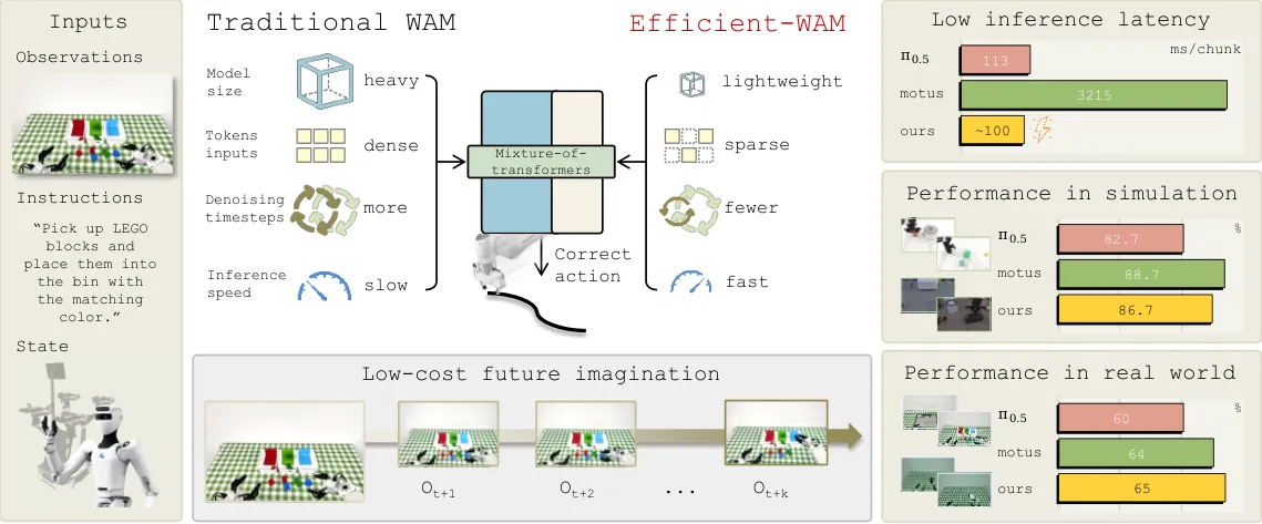
Figure 1 (paper Figure 1): overview of Efficient-WAM; the right panels report per-chunk latency (113 ms for pi0.5, 3215 ms for Motus, about 100 ms for this work) against simulation and real-world success.
In Table 1, the 1B Efficient-WAM reaches 86.7% clean and 85.7% randomized success, on par with the 4B LingBot-VLA (86.5/85.3) and the 5B GigaWorld-Policy (86.4/85.0), and only 2.0 points below the 8B Motus; Efficient-WAM-RT, with all efficiency mechanisms on, scores 83.1/82.0 and still exceeds pi0 (65.9/58.4) and StarVLA-alpha (76.8/79.1). Fast-WAM reports higher 91.9/91.8 but uses about six times the parameters, and this work runs faster while keeping future interaction at inference (Section 4.4 re-measures the original Fast-WAM at 381.6 ms per chunk under this protocol, versus 139 ms here). The numbers show that compression did not compress away control performance: in success per parameter, this model sits in the front row of Table 1.
| Method | Clean (%) | Random (%) | Params |
|---|---|---|---|
| pi0 | 65.9 | 58.4 | 3.3B |
| pi0.5 | 82.7 | 76.8 | 3.3B |
| LingBot-VLA | 86.5 | 85.3 | 4B |
| UWM | 81.7 | 78.6 | 5B |
| GigaWorld-Policy | 86.4 | 85.0 | 5B |
| Motus | 88.7 | 87.0 | 8B |
| Fast-WAM | 91.9 | 91.8 | 6B |
| Efficient-WAM | 86.7 | 85.7 | 1B |
| Efficient-WAM-RT | 83.1 | 82.0 | 1B |
Table 1 (paper Table 1, excerpt): RoboTwin 2.0 success rates; baseline numbers come from official papers or technical reports.
4.3 Real-world experiments
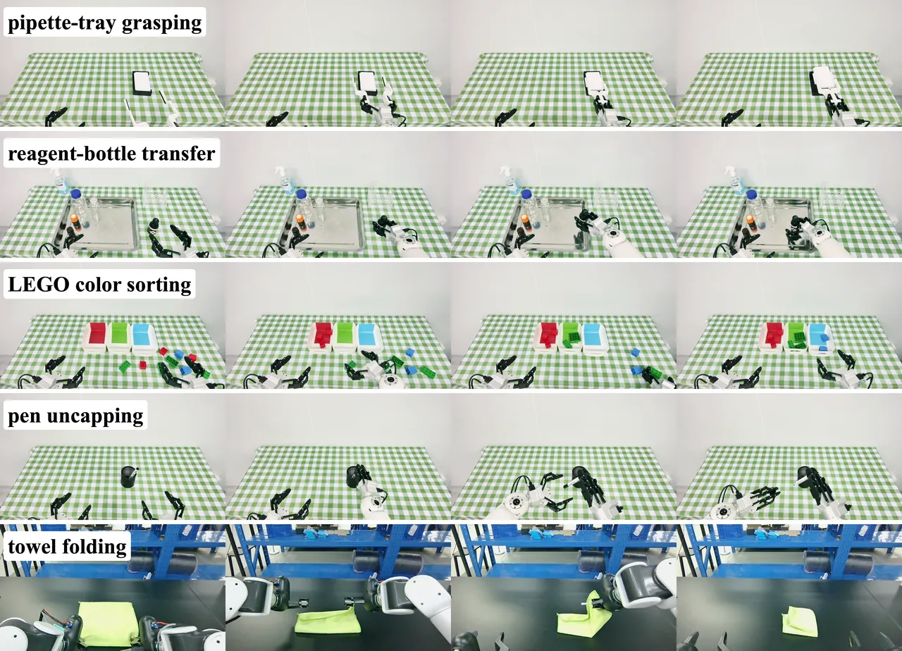
Figure 2 (paper Figure 3): five real-world tasks across two dual-arm platforms; the towel-folding main-camera view is recorded for visualization only and is not a policy input.
The real-world evaluation covers five tasks on two platforms (Figure 3 and Figure 5): the first four run on an Astribot S1 observing RGB from a head camera and both wrists with 31-dimensional joint states; towel folding runs on a separate dual-arm humanoid whose end effectors are Pika UMIs, where the policy sees only the two fisheye end-effector views and uses UMI relative-pose states and actions. pi0.5 is initialized from its official base checkpoint and Motus from WAN-2.2-5B, both fully fine-tuned; each method trains one policy per task on identical data (100 demonstrations per Astribot task, 1,000 UMI demonstrations for towel folding), with 20 trials per task and a three-minute limit per trial.
Efficient-WAM-RT averages 65.0% success across the five tasks (65 of 100 trials), above Motus at 64.0% and pi0.5 at 60.0%, at 98 ms per chunk on an RTX 4090, i.e. 6.1 ms amortized over the 16 actions, versus 3215 ms and 200.9 ms for Motus, more than 30x faster in the same deployment setup. Per task, this work is best at pen uncapping (30%), ties Motus on LEGO color sorting (65%, where pi0.5 manages only 30%), but trails pi0.5 on pipette-tray grasping (95 vs 100) and is last on towel folding (60%, pi0.5 at 85%). The average advantage comes mainly from rigid-object tasks; deformable manipulation remains the weak spot, which the limitations section revisits.
| Real-world task | pi0.5 | Motus | Ours |
|---|---|---|---|
| pipette-tray grasping | 100.0 | 85.0 | 95.0 |
| reagent-bottle transfer | 75.0 | 80.0 | 75.0 |
| LEGO color sorting | 30.0 | 65.0 | 65.0 |
| pen uncapping | 10.0 | 25.0 | 30.0 |
| towel folding (dagger) | 85.0 | 65.0 | 60.0 |
| Avg. success rate (%) | 60.0 | 64.0 | 65.0 |
| Avg. latency per chunk (ms) | 113.0 | 3215.0 | 98.0 |
| Amortized latency per action (ms) | 7.1 | 200.9 | 6.1 |
Table 2 (paper Table 2): real-world evaluation; the dagger task uses a separate robot platform and setup, and RTX 4090 latency is reported per chunk and amortized over 16 actions.
4.4 Ablations: what each factor is worth
Is future interaction necessary? The authors build FastMask, Fast-WAM's attention mask and inference scheme ported to this MoT, as the control that keeps video co-training but skips future generation at inference (Table 3). In paired comparisons where backbone, action expert, training data, optimization, and evaluation protocol are identical, removing future interaction drops Efficient-WAM from 86.7/85.7 to 65.8/65.6, a loss of 20.9 and 20.1 points; the full WAM-5B also drops at both batch sizes but less severely. The original Fast-WAM re-measured under this protocol takes 381.6 ms per chunk. Two conclusions follow: under this MoT configuration future interaction is load-bearing and Fast-WAM's inference design is not a drop-in replacement, while this work keeps that interaction at 139 ms, faster than the original Fast-WAM.
| Model (batch size) | Future interaction | FastMask |
|---|---|---|
| WAM-5B (16x16) | 86.4 / 85.5 | 76.9 / 73.8 |
| WAM-5B (16x64) | 88.0 / 89.4 | 83.1 / 83.3 |
| Efficient-WAM (16x8) | 86.7 / 85.7 | 65.8 / 65.6 |
Table 3 (paper Table 3): future-interaction ablation, clean and randomized success rates.
Compact expert and resolution. Table 4a trains the video expert from scratch as a control: random initialization gives 69/68, structured slicing raises it to 82/81, and teacher distillation further to 87/86, close to the full backbone's 86.4/85.5, while per-chunk latency falls from 2013 ms to 430 ms. Slicing and distillation contribute roughly 13 and 5 points respectively, showing that pretrained initialization and distillation preserve world priors after compression. In Table 4b, future tokens drop from 240 to 126 to 60 with latency 430, 396, 377 ms and success 87/86, 85/84, 83/82: one quarter of the tokens costs about 4 points, the best price among the three factors.
| Video expert variant | Init. | Distill | Clean / Rand (%) | Latency (ms/chunk, A800) |
|---|---|---|---|---|
| Full WAN (5B) | full teacher | - | 86.4 / 85.5 | 2013 |
| Compact random init | random | no | 69 / 68 | 432 |
| Compact sliced | structured slice | no | 82 / 81 | 426 |
| Efficient-WAM | structured slice | yes | 87 / 86 | 430 |
Table 4 (paper Table 4a): initialization and distillation ablation for the compact video expert; parameters count only the video expert.
Asymmetric denoising. Figure 4 sweeps the $[T_{v},T_{a}]$ configuration: going from [10,10] at 431 ms and 87.1% to [2,10] at 139 ms and 86.3% buys a 3.1x latency reduction for only 0.8 points; moving the two video updates to action iterations 1 and 8 (the starred [2,10] variant) gives 140 ms and 86.2%, statistically indistinguishable from the default, so the first two iterations become the default schedule. More aggressive video budgets hurt clearly: [1,10] gives 92 ms and 79.3%, [2,2] gives 101 ms and 84.1%. This curve is the most persuasive figure in the paper: it turns the number of video updates from an architectural constant into a tunable knob and marks the knee.
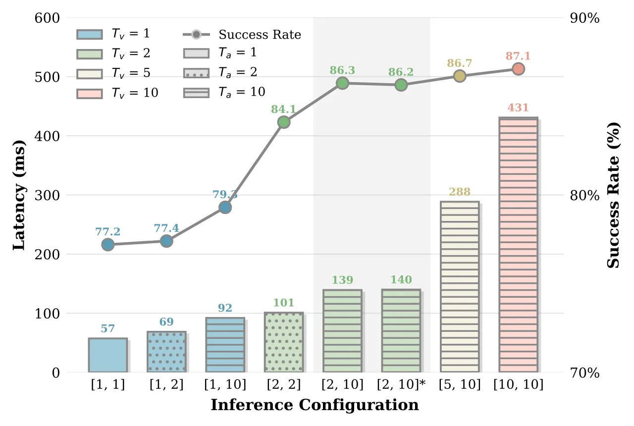
Figure 3 (paper Figure 4): latency-success trade-off on RoboTwin 2.0 (clean); shading marks the selected [2,10] configuration and the star marks the variant updating video at iterations 1 and 8.
4.5 Decoupling fidelity from control
To test the central claim directly, the authors run video-only generation on the RoboTwin hanging_mug task without the action expert and compare prediction fidelity of the compact 0.8B expert against the full WAN-2.2-5B (Table 5): PSNR falls from 21.66 dB to 18.82 dB and SSIM from 83.18% to 79.16%, so the compressed futures are indeed coarser (the qualitative comparison in Figure 7 and Figure 8 shows the same). Yet the same compact expert keeps control success close to the full backbone (Table 4a). Coarser video and undegraded control holding simultaneously is the empirical form of the design philosophy: the future branch exists to guide actions, not to produce viewable footage.
| Model | PSNR (dB), higher better | SSIM (%), higher better |
|---|---|---|
| WAM-5B | 21.66 | 83.18 |
| Efficient-WAM | 18.82 | 79.16 |
Table 5 (paper Table 5): future-prediction fidelity of the video branch alone on RoboTwin hanging_mug.
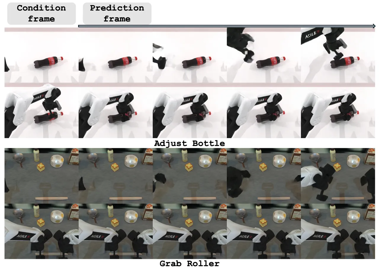
Figure 4 (paper Figure 7): future predictions of the full-backbone WAM-5B on two RoboTwin tasks.
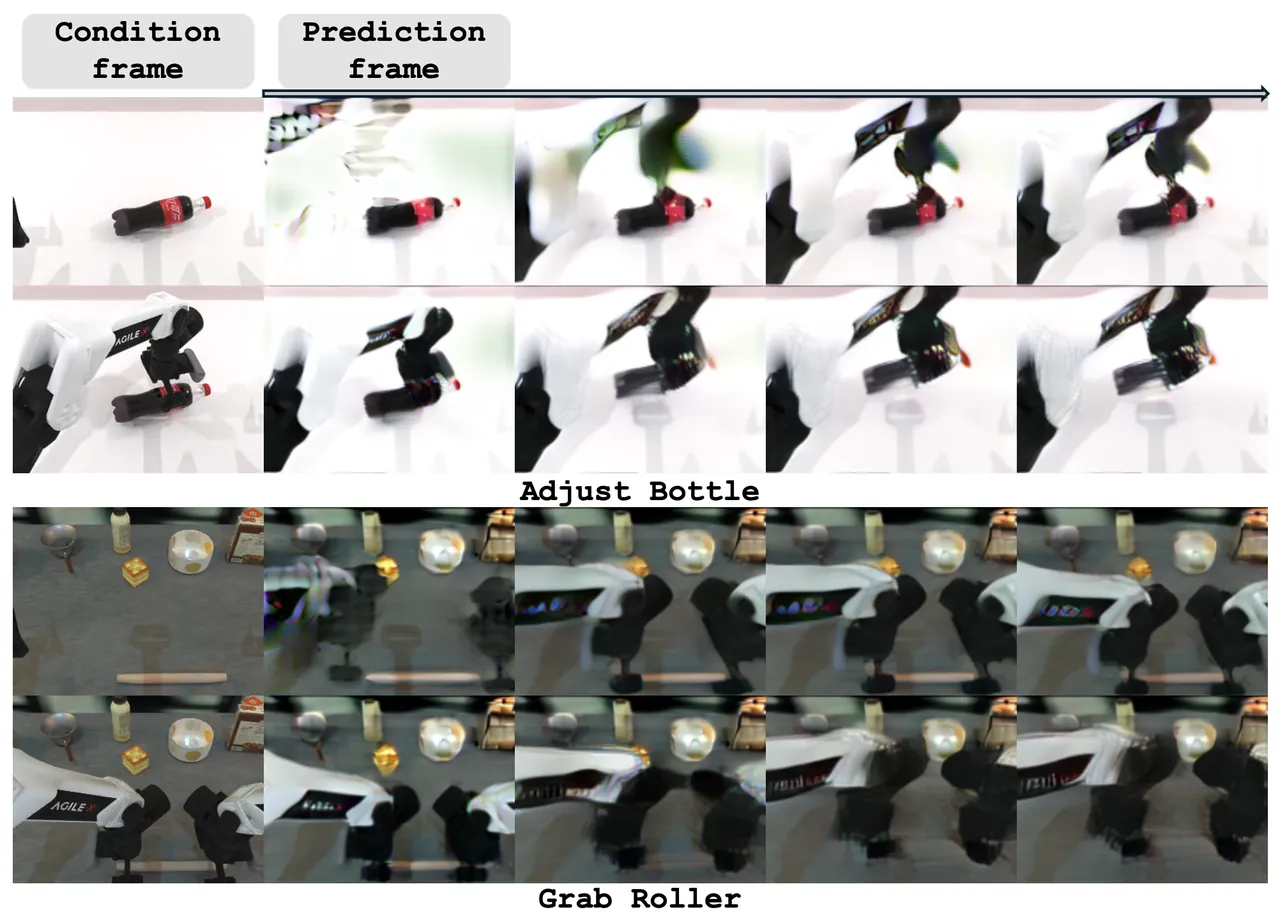
Figure 5 (paper Figure 8): future predictions of Efficient-WAM-RT, visibly coarser while control success stays close.
The failure study (Figure 6) shows three failure families shared by all models: grasp misalignment, overlooked objects, and unintended collisions. Failures specific to pi0.5 include leaving LEGO blocks unsorted and toppling the pen holder, which the authors attribute to incomplete task adaptation with only 100 demonstrations; the specific risk for the two WAMs is sensitivity to visual differences between UMI collection and deployment, since all towel demonstrations come from a single Pika UMI setup and, despite matching camera models and settings, the robot-mounted cameras produce different images and VAE latents at approximately matched viewpoints.
5. Limitations
Author-stated, first: the resolution-for-speed boundary is uncharted. Low-resolution future prediction trades visual detail for inference speed; the authors state explicitly that tasks requiring finer spatial precision, such as thread insertion, may still benefit from higher-resolution future representations, and that this trade-off remains unevaluated in such settings.
Author-stated, second: camera appearance shift. The visual differences observed between UMI collection and deployment (different images and VAE latents at approximately matched viewpoints despite identical camera models and settings) motivate further study of robustness to camera variation; the towel-folding demonstrations come from a single Pika UMI setup, the direct source of that shift.
Our assessment, first: the deformable-object evidence is narrow and lands on the weak spot. The real-world protocol uses 20 trials per task, and among the five tasks only towel folding involves a deformable object, precisely the task where Efficient-WAM-RT (60%) trails pi0.5 (85%). The average-success advantage is therefore carried by rigid-object tasks, the claim of deformable-object support rests on thin evidence, and the authors' appearance-shift explanation is a confounded candidate cause that the experiments cannot separate.
Our assessment, second: latency accounting and baseline protocols. The 98 ms deployment figure excludes predicted-video VAE decoding and saving as well as observation acquisition and robot execution; any downstream use that visualizes predicted futures or closes a loop on them would see a higher end-to-end wall clock. Ablations run on an A800 while deployment runs on an RTX 4090, so the two hardware regimes should not be multiplied into a single extrapolation, and most Table 1 baselines come from official papers or reports rather than re-runs under one protocol (Fast-WAM excepted), leaving protocol variance in cross-method comparisons.
6. Conclusion and Outlook
Efficient-WAM amounts to a cost decomposition followed by per-factor compression and combined validation: Equation (2) splits video-side cost into model size, token count, and denoising steps; a sliced-and-distilled 0.8B compact expert, one-quarter future tokens at 192x160, and training-free [2,10] asymmetric denoising answer the three factors; RoboTwin 2.0 and real-robot experiments validate the combination. The ablations also supply the negative evidence that removing future interaction costs about 20 points, showing that what gets compressed is the resolution and the step count of imagination, not imagination itself.
For robot learners the reusable assets are three: a slicing-and-distillation recipe that cuts a 30-layer video teacher to 12 layers while keeping its priors; an inference pattern of cached video K/V plus action-only refinement that transfers to other MoT-style WAMs; and a latency-success curve with a marked knee that deployment budgets can read off directly. The outlook follows the two author-stated gaps: resolution requirements of fine-spatial-precision tasks, and robust training across camera appearance shifts.