PhyLatent: Learning Dynamics-Relevant Representations for JEPA World Models

Authors: Xi Zeng, Haojie Ren, Ziying Song　Source: arXiv:2608.05720　Date: 2026-08-06

Code status: The authors do not provide an official public PhyLatent repository. Experiments use the datasets and interfaces from stable-worldmodel, and the LeWorldModel baseline is available through le-wm.

Background and Motivation

Joint-Embedding Predictive Architectures are built around a simple premise: predictive learning should occur in a compact representation space rather than by reconstructing pixels. JEPA first emerged as a general approach for self-supervised image and video prediction, and recent action-conditioned variants extend it to embodied planning and control.

LeWorldModel is the direct baseline in this paper. It encodes pixel observations into latent vectors, uses an action-conditioned predictor to produce future latents, and applies Sketched Isotropic Gaussian Regularization (SIGReg) to keep the aggregate latent distribution non-degenerate. This setup allows model predictive control to rank action sequences directly in the learned latent space.

The central observation is that a globally non-collapsed latent distribution does not guarantee a locally meaningful state space. The overall point cloud can be well spread while nuisance appearance changes dominate real transitions, physically distinct states remain folded together, or predicted futures from different actions stay too close to support reliable action comparison.

The paper names these three problems physical invariance collapse, physical identifiability collapse, and counterfactual dynamics collapse. Each is defined by an explicit criterion and measured with a diagnostic set sampled from the Cube environment. Figure 1 summarizes all three failure modes and the desired latent geometry.

PhyLatent does not replace the JEPA backbone or the planner. Instead, it attaches training-time constraints to the shared prediction graph and removes all auxiliary heads after training, so the inference model has the same computational cost as the baseline while learning a more useful latent geometry.

Related Work and Problem Positioning

The JEPA line has grown from masked image prediction to spatiotemporal video prediction and action-conditioned world models. I-JEPA predicts abstract representations of masked regions, V-JEPA extends that idea to video, V-JEPA 2 and LeWorldModel support planning, and SD-JEPA decomposes latent space into progression and content subspaces. These models avoid pixel reconstruction but still inherit the question of whether the latent geometry preserves the state variables that control future evolution.

Representation-collapse methods address the failure mode in which joint embedding models output a constant or low-rank representation. Contrastive objectives, asymmetric prediction, momentum targets, redundancy reduction, and variance-covariance regularization all promote a healthier aggregate distribution. SIGReg adapts this idea to end-to-end world models, while Sub-JEPA relaxes the Gaussian constraint over random subspaces. None of these methods specifies which sample pairs should be invariant or how far physically distinct futures should be separated.

Dynamics-aware representation learning has a longer history in control. Time-contrastive networks, DeepMDP, inverse-dynamics regularization, and Sensorimotor World Models try to retain task-relevant dynamics while discarding irrelevant appearance. PhyLatent occupies a complementary position: it converts three local geometric requirements into explicit training objectives on the shared JEPA graph rather than relying on aggregate statistics or pointwise prediction error alone.

Preliminaries

The single-transition LeWorldModel graph is captured by Eq. (1). The encoder $E$ and projection head $P$ map observations to latents, while the action-conditioned predictor $F_\theta$ produces the future latent from the current latent and action:

$$z_t=P(E(o_t)),\quad z_{t+1}=P(E(o_{t+1})),\quad \hat{z}_{t+1}=F_\theta(z_t,a_t).$$

The baseline objective in Eq. (2) matches the predicted future latent to a stop-gradient copy of the encoded future latent:

$$\mathcal{L}_{\mathrm{pred}}=\left\|\hat{z}_{t+1}-\mathrm{sg}(z_{t+1})\right\|_2^2.$$

SIGReg regularizes the aggregated latent distribution, but it does not prescribe which pairs should be invariant, which physical states should be separated, or how action-conditioned futures should be organized. Because MPC evaluates candidate actions through distances between predicted latent trajectories, local geometry is not a cosmetic detail; it directly determines whether the planner can compare futures.

Method

PhyLatent operates on a shared sequence-level training graph. Given an observation sequence $O$, raw action sequence $A$, encoded latent sequence $Z$, and target future $Z^{+}$, the predictor produces $\hat{Z}$. The sequence objective is defined with a normalized mean-squared distance $d_N$, and the baseline remains $\mathcal{L}_{\mathrm{pred}}$. Three pathways are attached to this graph.

The normalized distance normalizes each tensor independently along the final feature dimension before computing the mean squared difference:

$$d_N(X,Y)=\operatorname{mean}\left[\left(\operatorname{norm}_{-1}(X)-\operatorname{norm}_{-1}(Y)\right)^2\right].$$

This shared scale makes the auxiliary losses comparable across latent features and reduces sensitivity to per-dimension variance, which matters because several objectives operate on the same 192-dimensional representation.

flowchart TB
    subgraph Shared["Shared JEPA Backbone"]
        O[Observation Sequence] --> E[Encoder + Projection]
        A[Action Sequence] --> AE[Action Encoder]
        E --> Z[Latent Sequence Z]
        AE --> C[Action Embedding C]
        Z --> F[Action-Conditioned Predictor]
        C --> F
        F --> PZ[Predicted Future Z-hat]
    end
    subgraph Invariance["Physical Invariance"]
        OA[Augmented Observation] --> E
        E --> ZA[Augmented Latent Z-aug]
        ZA --> SVIC[SVIC Aligns to Stop-Gradient Z]
    end
    subgraph Identifiability["Physical Identifiability"]
        Z --> PSG[PSG Predicts Physical Targets]
        PZ --> PSG2[PSG Predicts Physical Targets]
        Z --> FRA[FRA: Projection + Action-Query Alignment]
        PZ --> FRA
    end
    subgraph Counterfactual["Counterfactual Dynamics"]
        A --> CA[Permuted Actions + Noise]
        CA --> F2[Predictor Produces Counterfactual Branch]
        F2 --> CASC[CASC Separates Action Branches]
        PZ --> LD[LD Denoises Future Latents]
    end
    Shared --> Invariance
    Shared --> Identifiability
    Shared --> Counterfactual

Physical Invariance: SVIC

Physical invariance requires observations with the same simulator state to remain close after appearance-only changes. The paper applies brightness and per-channel perturbations, then compares the nuisance displacement $d_{\mathrm{nuis}}$ with the displacement caused by a real transition $d_{\mathrm{state}}$:

$$d_{\mathrm{nuis}}=\left\|z_t-z_t^{\mathrm{aug}}\right\|_2,\quad d_{\mathrm{state}}=\left\|z_t-z_{t+\Delta}\right\|_2,\quad \mathcal{C}_{\mathrm{inv}}: d_{\mathrm{nuis}}>d_{\mathrm{state}}.$$

Equation (4) is both the diagnostic criterion and the motivation for SVIC. The Static Visual Invariance Constraint aligns the augmented sequence to a stop-gradient copy of the original sequence:

$$\mathcal{L}_{\mathrm{inv}}=d_N\left(Z^{\mathrm{aug}},\mathrm{sg}(Z)\right).$$

The stop-gradient keeps the original sequence as a stable reference while gradients update the augmented branch. Unlike global distribution regularization, SVIC directly suppresses nuisance-driven movement in the representation consumed by the dynamics predictor, which is the geometry that ultimately influences MPC.

Physical Identifiability: PSG and FRA

Physical identifiability requires physically distinct robot-object configurations to remain separated. Physical State Grounding (PSG) applies a shared state head $H_s$ to both the encoded trajectory and the predicted continuation, regressing normalized simulator-derived physical targets:

$$\mathcal{L}_{\mathrm{state}}=\operatorname{MSE}\left(H_s(Z),\bar{S}\right)+\operatorname{MSE}\left(H_s(\hat{Z}),\bar{S}_{K+1:T}\right).$$

PSG targets are task-specific. Cube uses a 28-dimensional target covering arm joints, end-effector pose, gripper state, and cube state; TwoRooms uses only the 2D agent position; PushT uses agent and block positions, angle, and velocities. The shared head gives encoded and predicted latents a common physical interpretation without exposing physical targets to the planner.

Future Representation Alignment (FRA) constrains the remaining structure of the predicted future. The projection branch uses a shared head $\phi$:

$$\mathcal{L}_{\mathrm{proj}}=d_N\left(\phi(\hat{Z}),\mathrm{sg}\left(\phi(Z^{+})\right)\right).$$

The action-query branch summarizes the context action embedding into a query and applies multi-head attention over the latent sequence, aligning the future structure selected by the executed action:

$$\mathcal{L}_{\mathrm{act}}=d_N\left(\Psi(\hat{Z},C_{\mathrm{ctx}}^{a}),\mathrm{sg}\left(\Psi(Z^{+},C_{\mathrm{ctx}}^{a})\right)\right).$$

These two branches are combined into $\mathcal{L}_{\mathrm{align}}$. Together, PSG and FRA prevent the model from learning a representation that is merely non-collapsed while still folding distant physical states into the same local neighborhood.

Counterfactual Dynamics: CASC and LD

MPC needs to distinguish the consequences of different actions. Counterfactual Action Separation Constraint (CASC) constructs a counterfactual action sequence by permuting actions across the mini-batch and adding Gaussian noise, then generates a counterfactual future branch with the same predictor. The separation objective uses a hinge term with a margin proportional to action difference:

$$\mathcal{L}_{\mathrm{sep}}=\frac{1}{|\Omega|}\sum_{(b,\tau)\in\Omega}\left[m_{b,\tau}-\delta_{b,\tau}^{z}\right]_{+},\quad [x]_{+}=\max(x,0).$$

CASC keeps only temporal positions whose action difference exceeds the batch median, so nearly identical actions are not forced apart. The factual branch is a stop-gradient reference; the counterfactual branch is pushed away without globally expanding the latent space without bound.

Latent Denoising (LD) regularizes the local structure around future latents. Noise is added to a detached target future, and a denoising head receives the noisy future, the predicted future, action conditioning, and noise scale. Its objective is $\mathcal{L}_{\mathrm{denoise}}=\operatorname{MSE}(\hat{\epsilon},\epsilon)$, which encourages the predicted future to lie in a locally regular, denoising-friendly region without pixel reconstruction.

The complete training objective combines all pathways with task-dependent weights:

$$\mathcal{L}_{\mathrm{PhyLatent}}=\mathcal{L}_{\mathrm{pred}}+0.09\mathcal{L}_{\mathrm{SIGReg}}+\lambda_{\mathrm{inv}}\mathcal{L}_{\mathrm{inv}}+\lambda_{\mathrm{state}}\mathcal{L}_{\mathrm{state}}+\lambda_{\mathrm{align}}\left(\mathcal{L}_{\mathrm{proj}}+\mathcal{L}_{\mathrm{act}}\right)+\lambda_{\mathrm{sep}}\mathcal{L}_{\mathrm{sep}}+\lambda_{\mathrm{denoise}}\mathcal{L}_{\mathrm{denoise}}.$$

After training, only the encoder, projection head, action encoder, and predictor are exported. State heads, alignment heads, the action-query module, and the denoiser are removed, so inference-time computation and the MPC planner are unchanged.

Experimental Results

Experiments use the standardized datasets and interfaces from stable-worldmodel. Cube is an offline goal-conditioned manipulation task, TwoRooms is visual navigation across connected rooms, Reacher is a joint reaching task, and PushT is contact-rich planar pushing. The encoder is a ViT-Tiny with patch size 14, latent dimension 192, and a six-block action-conditioned Transformer predictor.

Task	Transitions	Episodes	Avg. Steps / Episode	Size
Cube	2,010,000	10,000	201.00	94.94 GiB
TwoRooms	920,809	10,000	92.08	11.90 GiB
Reacher	2,010,000	10,000	201.00	92.11 GiB
PushT	2,336,736	18,685	125.06	43.12 GiB

Evaluation follows a fixed protocol. Each rollout starts from a sampled dataset state and sets the goal to the state 25 steps later in the same trajectory, with a maximum of 50 environment steps. One hundred episodes are evaluated per random seed, and results are averaged over three seeds. Success thresholds are task-specific: Cube requires the object to reach the target radius, TwoRooms requires arrival within 16 pixels, Reacher checks joint errors, and PushT checks both position and angle.

PhyLatent uses unit weight for the prediction loss, 0.09 for SIGReg, and task-specific weights for the five auxiliary objectives. The weights reveal a practical tradeoff: Cube and TwoRooms rely more heavily on PSG, while Reacher and PushT use smaller auxiliary coefficients. Simply increasing physical supervision on contact-heavy tasks does not resolve their planning failures.

Task	PSG	FRA	SVIC	CASC	LD
Cube	0.25	0.10	0.05	0.02	0.01
TwoRooms	0.20	0.08	0.03	0.02	0.01
Reacher	0.045	0.025	0.030	0.015	0.005
PushT	0.090	0.035	0.060	0.010	0.005

The proposed diagnostics are evaluated on Cube. Physical invariance uses 1,000 states, physical identifiability uses 200,000 state pairs, and counterfactual dynamics uses 1,000 action pairs. The JEPA+SIGReg baseline fails 15.60%, 6.71%, and 8.41% of these cases. Figure 1 explains the three failure geometries, and Figure 2 visualizes them as three-dimensional point clouds with decision boundaries.

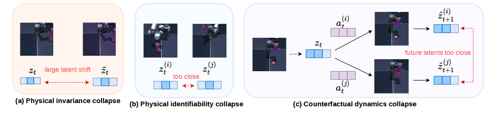
Figure 1: Three locally collapsed latent geometries that a globally non-collapsed distribution can still contain.

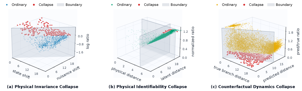
Figure 2: Three-dimensional diagnostics of LeWorldModel on Cube; red points satisfy the corresponding collapse criterion.

PhyLatent lowers the Cube failure rates to 7.53%, 0.95%, and 4.62%, and raises MPC success from 70.00%±4.00 to 78.10%±2.80. Figure 3 shows the shared backbone and the three training pathways, while Figure 4 compares the baseline and PhyLatent on the same diagnostic sets.

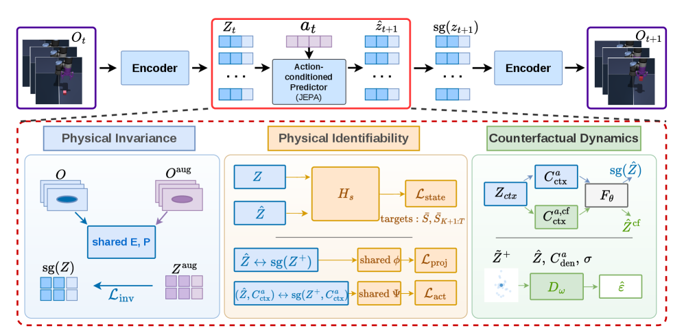
Figure 3: Shared action-conditioned JEPA backbone with the three PhyLatent training pathways.

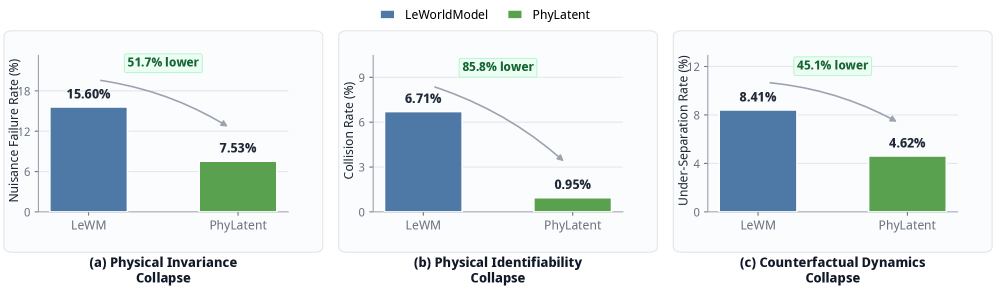
Figure 4: Dynamics-relevant collapse reduction on Cube for JEPA+SIGReg versus PhyLatent.

Planning results show that the same representation principles transfer across manipulation and navigation. TwoRooms improves from 81.00%±6.24 to 98.00%±1.00, and Reacher improves from 78.33%±2.08 to 79.33%±3.51. PushT decreases slightly from 77.67%±0.58 to 75.33%±2.08, making it the most informative negative result in the paper.

Task	JEPA + SIGReg	PhyLatent
Cube	70.00 ± 4.00	78.10 ± 2.80
TwoRooms	81.00 ± 6.24	98.00 ± 1.00
Reacher	78.33 ± 2.08	79.33 ± 3.51
PushT	77.67 ± 0.58	75.33 ± 2.08

The grouped ablation isolates each pathway on Cube. Removing PSG and FRA raises counterfactual failure to 6.84% and lowers success to 74.00%. Removing SVIC raises invariance failure to 9.93%. Removing CASC and LD produces the largest planning drop, to 73.33%. The complete objective achieves the best tradeoff across diagnostics and planning.

Method	Inv. Fail.	Id. Fail.	CF Fail.	Success
JEPA + SIGReg	15.60	6.71	8.41	70.00 ± 4.00
PhyLatent	7.53	0.95	4.62	78.10 ± 2.80
w/o PSG + FRA	7.17	1.03	6.84	74.00 ± 1.00
w/o SVIC	9.93	0.84	4.26	77.00 ± 1.00
w/o CASC + LD	12.77	0.78	4.74	73.33 ± 3.51

The ablation also shows that diagnostic rates alone do not fully explain planning quality. Removing CASC and LD changes the counterfactual diagnostic only slightly, from 4.62% to 4.74%, yet causes the largest planning drop. This suggests the pair contributes to local future geometry in ways that the single counterfactual failure metric does not capture.

The appendix provides a useful boundary case on PushT. PhyLatent reduces the three diagnostics from 1.33%, 1.15%, and 4.25% to 0.20%, 0.52%, and 2.38%, yet planning success does not improve. The authors interpret this as evidence that contact-rich pushing additionally depends on precise local contact transitions and the geometry of the planning objective.

Method	Inv. Fail.	Id. Fail.	CF Fail.
JEPA + SIGReg	1.33	1.15	4.25
PhyLatent	0.20	0.52	2.38

A threshold sensitivity analysis addresses the concern that the identifiability diagnostic depends on arbitrary quantiles. Across nine combinations of physical-distance and latent-neighborhood thresholds, PhyLatent achieves a lower collision rate than JEPA+SIGReg in every setting, and at the default thresholds it lowers the rate from 6.71% to 0.95%.

Figure 5 aligns with these numbers at the behavioral level. In the baseline rollout, the gripper makes initial contact but loses the cube during execution. PhyLatent maintains contact and transports the cube through later time steps. This qualitative result connects the latent diagnostics to a concrete manipulation failure mode.

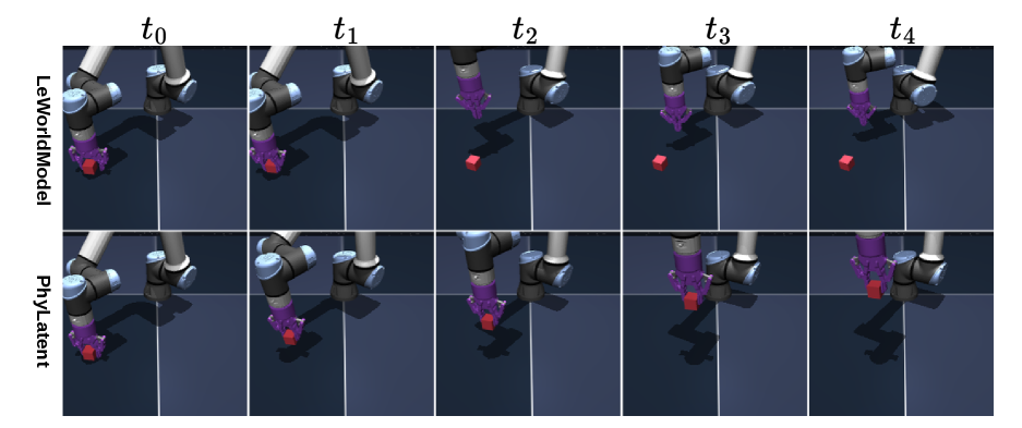
Figure 5: Representative Cube MPC rollouts: JEPA+SIGReg loses contact, while PhyLatent maintains the robot-object interaction.

Discussion and Limitations

The authors state one clear limitation: PhyLatent requires task-specific physical targets as auxiliary supervision during training. These targets are natural in simulators, but may not be available for real robots, raw video collections, or open-world tasks. The stated future direction is to find broader supervision signals while preserving dynamics-relevant structure.

From a design perspective, PhyLatent is attractive because it leaves the inference-time JEPA and MPC unchanged. It upgrades the learning objective rather than the planner, and its diagnostics give concrete criteria for what a state-space representation should preserve. The cost is added complexity and task-specific tuning of five loss weights, which differ across Cube, TwoRooms, Reacher, and PushT.

Independently, the PushT result is the most important boundary. Improved diagnostic rates do not automatically translate into better control, so the proposed constraints may overfit the structure measured by the diagnostics while leaving other aspects of contact-rich dynamics untouched. The absence of official code also limits reproducibility, and the diagnostic protocol itself requires access to simulator states or standardized physical targets.

Future work could weaken the dependence on explicit physical states by learning inverse-dynamics or weak-label alternatives, extend CASC beyond within-batch permutations to cross-environment counterfactuals, and jointly optimize representation diagnostics with the planning objective.

Reproduction cost is also a practical constraint. Training uses bfloat16 on a single RTX 5080 and takes roughly 14 hours 35 minutes for Cube, 3 hours 32 minutes for TwoRooms, 19 hours 2 minutes for Reacher, and 32 hours 43 minutes for PushT. Real-robot deployment would add the harder problem of obtaining task-specific physical targets from non-simulator data.

The method can also be interpreted from the planner's perspective. MPC samples 100 candidate action sequences, keeps the top 10 elites, and evaluates them through predicted latent trajectories. SVIC stabilizes the goal representation, PSG and FRA keep predicted trajectories aligned with physical positions, and CASC with LD keep alternative futures comparable. Each pathway addresses a distinct failure point on this control loop.

Conclusion

PhyLatent reframes JEPA world-model learning from global distributional health to dynamics-relevant local geometry. By adding SVIC, PSG, FRA, CASC, and LD as training-only constraints, it reduces all three diagnosed collapse rates on Cube and improves MPC on both manipulation and navigation benchmarks.

The broader lesson is that world-model evaluation should not stop at reconstruction error, pointwise prediction loss, or global non-collapse. A reliable latent state space must also preserve physical invariance, state identifiability, and action-conditioned future separation. PhyLatent turns those properties into measurable diagnostics and trainable objectives, while leaving the harder problem of contact-rich control visible for future work.