Learning Agile Navigation in Crowded Environments for Quadruped Robots

Paper Overview

Title: Learning Agile Navigation in Crowded Environments for Quadruped Robots
Authors: Shuyu Wu, Zeyu Liu, Tianbao Zhang, Fanxing Li, Fangyu Sun, Mingkang Xiong, Wei Xi, Wenxian Yu, Danping Zou
Affiliations: Shanghai Jiao Tong University; State Key Laboratory of High-end Heavy-load Robots, Midea Group
arXiv: 2607.15036 (v1, 16 Jul 2026)
Code: no public repository is provided by the authors as of this writing.

One-sentence summary: VOP-Nav teaches a quadruped robot to sprint through crowds by training a lightweight perception network (VOP-Net) to regress Velocity-Obstacle-style safe velocity intervals directly from five frames of raw LiDAR — no detection, no tracking — and then feeding those predictions to the navigation policy both as observations and as a reward signal.

1. Background and Motivation

Quadruped robots destined for city streets, shopping malls, factories, or transit hubs must share space with people. Crowds are hostile to perception: pedestrians occlude one another and occlude the robot's sensors, and their future trajectories are hard to predict. The stakes are highest in time-critical missions. The paper opens with the image of a firefighting scenario in which a robot must carry emergency supplies through a counter-flow of evacuees; if the robot hesitates, the mission stalls. The design objective is therefore a system that is simultaneously safe (zero collisions) and agile (fast enough to exploit transient gaps before they close).

The classical solution is the perception-planning-control pipeline. Planners such as the Dynamic Window Approach or Velocity Obstacle (VO) methods reason in velocity space and can impose explicit collision-avoidance constraints. Their weakness is the assumption they run on: accurate position and velocity estimates for every obstacle. Prior work either grants the planner privileged ground-truth obstacle states (unavailable outside simulation) or bolts on detection and tracking modules — YOLO detectors, multi-hypothesis trackers — to estimate those states from onboard sensors. In dense crowds, occlusion and noise make such estimates unreliable, and a VO planner fed with bad states makes bad decisions.

The alternative is end-to-end learning: a policy trained by reinforcement learning or differentiable physics maps raw sensor observations straight to joint-level commands. End-to-end systems skip fragile intermediate modules and, for legged robots, can exploit the full agility of the platform. Yet the authors' own experiments show that end-to-end policies degrade in dense dynamic scenes. They attribute this to two related problems. First, reward design: conventional collision or distance penalties only teach reactive dodging, not the foresight to stay away from regions that are about to become dangerous. Second, representation: a policy that consumes only raw sensor streams has no explicit structure for encoding time-varying collision constraints imposed by moving obstacles.

The paper's diagnosis is that both camps are right about one thing and wrong about another. Model-based VO methods have the right safety abstraction but the wrong perception interface; end-to-end methods have the right perception interface but no safety abstraction. VOP-Nav's proposal is to keep the VO abstraction — a safe velocity region in the robot's own velocity space — while discarding the assumption that obstacles must first be detected and tracked. Instead, a neural network learns to perceive the safe velocity region directly from multi-frame LiDAR data. The authors call this idea "Velocity Obstacle Perception".

Three contributions are claimed: (1) VOP-Nav, a unified end-to-end framework that integrates VO principles with reinforcement learning using only local observations, without maps, detection, or tracking; (2) VOP-Net, the perception network that predicts the safe velocity region; and (3) an Isaac Gym simulation framework populated with diverse dense dynamic scenarios for training and generalization evaluation. The trained policy deploys zero-shot on a Unitree Go2 and works indoors and outdoors with onboard sensing only.

2. Preliminaries: Velocity Obstacles

The VO formalism (following ORCA's presentation) starts with robot A modeled as a disc of radius $r_A$ and obstacle B as a disc of radius $r_B$. With the robot reduced to a point, the obstacle is inflated to the Minkowski sum disc $\hat{B}$ centered at $p_B$ with radius $r_A+r_B$. The collision cone collects all relative velocities whose ray from $p_A$ hits $\hat{B}$:

$$C_{AB}=\{v_{AB}\mid \lambda_{AB}\cap\hat{B}\neq\emptyset\}$$

where $v_{AB}=v_A-v_B$ is the relative velocity and $\lambda_{AB}$ the ray from $p_A$ along $v_{AB}$. Because the robot only cares about collisions within a planning horizon $\tau$, the cone is truncated by removing directions whose collision lies beyond $\tau$; the truncated cone is $CC_{AB}$. The velocity obstacle for A induced by B is then the truncated cone translated by the obstacle's own velocity:

$$\text{VO}^{\tau}_{A|B}=\{v_{A}\mid v_{A}\in CC_{AB}\oplus v_{B}\}$$

where $\oplus$ is the Minkowski sum. If the robot's velocity $v_A$ falls inside this translated cone, a collision happens within $\tau$. Non-circular obstacles (boxes, walls) are handled by extracting their corner points and treating each as a circular obstacle of radius $r_A$. This geometry is illustrated in the paper's Figure 3:

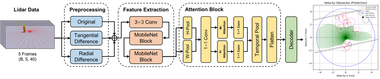
Figure 1: Geometry of the Velocity Obstacle. The beige truncated collision cone $CC_{AB}$ contains relative velocities that collide within horizon $\tau$; translating it by $v_B$ (gray region) yields $\text{VO}^{\tau}_{A|B}$ in absolute velocity space.

Two classical properties make VO attractive for crowds. It is local: each robot reasons only about nearby obstacles. And it converts a prediction problem ("where will that person be in two seconds?") into a geometric one about velocity directions. The catch, and the reason VO is rarely deployed raw on real robots in crowds, is that $v_B$ and $p_B$ must be known. VOP-Net exists precisely to produce the same safety information without estimating them.

3. Method: Three Training Stages

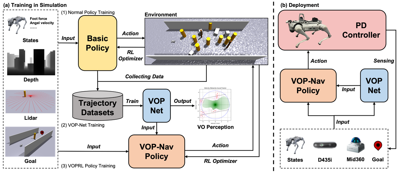
Figure 2: System architecture. (a) The three-stage simulation pipeline: Basic policy training, VOP-Net training on collected trajectories, and VOP-Nav policy training that consumes VOP-Net predictions as both input and reward. (b) Real-world deployment: VOP-Net and the VOP-Nav policy run concurrently at 50 Hz beside a 200 Hz PD controller.

The navigation task is formulated as a POMDP $\langle\mathcal{S},\mathcal{A},\mathcal{T},\mathcal{R},\Omega,\mathcal{O}\rangle$: the robot observes an occlusion-prone partial view through LiDAR, depth, and proprioception, and the objective is to maximize the discounted return $J(\pi_\theta)=\mathbb{E}_{\pi_\theta}\left[\sum_{t=0}^{\infty}\gamma^{t}r_{t}\right]$ with PPO. The system then trains in three stages, summarized in the flowchart below.

flowchart TD
    S1["Stage 1: Basic Policy
970-dim obs, 12-dim joint targets
PPO in Isaac Gym, 1024 envs"] -->|"rollouts in dynamic envs
10000 files x 1024 envs x 48 steps"| S2
    GT["Privileged simulator states
positions + velocities of all obstacles"] -->|"Algorithm 1: VO geometry"| LAB
    subgraph S2["Stage 2: VOP-Net"]
        LAB["360-degree safe intervals
(supervision signal)"]
        NET["5-frame LiDAR -> 3 channels
MobileNet + orthogonal attention
-> 360 x 2 safe intervals"]
    end
    S2 -->|"predictions as 720-dim input"| S3
    S2 -->|"r_VO soft constraint reward"| S3
    subgraph S3["Stage 3: VOP-Nav Policy"]
        POL["1693-dim obs -> 12-dim actions
trained from scratch"]
    end
    S3 -->|"zero-shot transfer"| REAL["Unitree Go2
Mid-360 LiDAR + D435i
50 Hz policy, 200 Hz PD"]

3.1 Stage 1 — the Basic policy

The Basic policy learns to walk and navigate in a dynamic simulation environment. Its observation vector has 970 dimensions: 50 proprioceptive dimensions (foot contact forces, base angular velocities, projected gravity vector, distance to goal, remaining episode time, joint positions and velocities, previous action), 880 exteroceptive dimensions from a 22×40 depth image, and a 40-dimensional LiDAR vector covering 360° at 9° resolution. The action is 12 target joint positions tracked by a PD controller with torque $\tau=K_{p}(t_{a}-q)-K_{d}\dot{q}$. Rewards are adapted from the ABS framework (collision penalties, goal tracking, torque and smoothness regularization), plus an agility reward that pays for fast goal-directed motion:

$$r_{\text{agile}}=\max\left\{\text{ReLU}\left(\frac{v_{x}}{v_{\text{max}}}\right)\cdot\mathbf{1}(\text{dir}_{\text{good}}),\ \mathbf{1}(d_{\text{goal}}<\sigma_{\text{tight}})\right\}$$

with $v_{\max}=4.5$ m/s, a heading-error gate of 105° for $\mathbf{1}(\text{dir}_{\text{good}})$, and a goal-proximity bonus that holds the reward once the robot is within $\sigma_{\text{tight}}=0.5$ m. The large $v_{\max}$ is deliberate: the Basic policy must physically be capable of high-speed maneuvers before safety constraints are layered on top.

3.2 Stage 2 — building the supervision signal and training VOP-Net

The supervision signal is the ground-truth safe velocity region, computed offline from privileged simulator states. Obstacle states are first transformed from the world frame to the robot's egocentric frame via the affine map $T_{R\rightarrow W}=\begin{bmatrix}R(\theta_R)&t\\0^T&1\end{bmatrix}$, with $R(\theta_R)=\begin{bmatrix}\cos\theta_R&-\sin\theta_R\\ \sin\theta_R&\cos\theta_R\end{bmatrix}$. Each obstacle contributes a VO region in robot velocity space; the union is $\Omega_{\text{VO}}=\bigcup_{i=1}^{n}\text{VO}_{O_i}$, and with the robot's maximum feasible speed set $V_{\max}$ (a disc of radius $v_{\max}$), the safe velocity region is

$$V_{\text{safe}}=V_{\max}\cap\overline{\Omega}_{\text{VO}}$$

A continuous safe region is awkward for network regression, so the angular space is discretized into $d=360$ directions. Along each ray $\lambda_j$, the algorithm measures the distance $L_j$ from the origin to the Minkowski boundary $\hat{B}$ (including tangency), sets the critical magnitude $D_j=\min(L_j,v_{\max})$, and emits a single interval per direction: $[0,D_j]$ if the robot is outside the VO region, or $[D_j,v_{\max}]$ if the robot is already inside the VO region — in which case the label tells the policy the minimum speed needed to escape the collision state. When a ray contains multiple disjoint safe segments, only the low-speed segment is kept, a conservative choice justified by the observation that learned locomotion cannot reliably track aggressive high-speed intervals. The final region is the element-wise intersection over all obstacles: $\mathbf{V}_{\text{safe}}=\bigcap_{i=1}^{n}\mathbf{V}^{O_i}_{\text{safe}}$. Algorithm 1 in the paper formalizes exactly this procedure.

The dataset consists of 10,000 files, each aggregating transitions from 1,024 parallel environments over 48 time steps, collected while the Basic policy navigated with $v_{\max}=4.5$ m/s. VOP-Net itself consumes the current LiDAR scan plus the four preceding frames, preprocessed into a three-channel tensor: raw distances, tangential (spatial) differences that highlight obstacle boundaries, and frame-to-frame radial (temporal) differences that encode relative motion cues. MobileNet blocks extract features; an orthogonal attention module pools separately along the time axis and the angular axis so the network can emphasize both critical past moments and hazardous directions; an MLP decoder regresses the $360\times 2$ interval output. The loss mixes an interval IoU term for geometric alignment with an MSE term for boundary precision:

$$\mathcal{L}=\alpha\,\mathcal{L}_{\text{IoU}}+(1-\alpha)\,\mathcal{L}_{\text{MSE}},\qquad \alpha=0.2$$

where, with $\mathbf{v}_{\text{pred}_j}$ and $\mathbf{v}_{\text{safe}_j}$ the predicted and ground-truth intervals on direction $j$, $\mathcal{L}_{\text{IoU}}=\frac{1}{d}\sum_{j=1}^{d}\left(1-\frac{|\mathbf{v}_{\text{pred}_j}\cap\mathbf{v}_{\text{safe}_j}|}{|\mathbf{v}_{\text{pred}_j}\cup\mathbf{v}_{\text{safe}_j}|+\epsilon}\right)$ and $\mathcal{L}_{\text{MSE}}=\frac{1}{2d}\sum_{j=1}^{d}\left((v^{\min}_{\text{pred}_j}-v^{\min}_{\text{safe}_j})^{2}+(v^{\max}_{\text{pred}_j}-v^{\max}_{\text{safe}_j})^{2}\right)$. On the validation set the trained VOP-Net reaches an IoU of 0.808 and an MSE of 0.172.

3.3 Stage 3 — the VOP-Nav policy

A design decision worth pausing on: VOP-Net's predictions are not enforced as hard constraints at runtime the way a classical VO safety filter would. Learned approximations from raw sensors carry bias and uncertainty, and clamping the robot's velocity to them could produce over-conservative or infeasible behavior. Instead the predictions shape the policy from the inside, in two complementary ways.

First, as observation: the observation space grows from the Basic policy's 970 dimensions to 1,693 by adding the robot's 3-dimensional linear velocity and the VOP-Net output flattened into 720 dimensions (min and max safe speed over 360 angles). Second, as reward: a velocity-constraint term penalizes commanded velocities that violate the predicted safe interval for the current heading, computed by inverse-distance interpolation over the $k=5$ nearest angular sectors with wrap-around angular distance $\delta_i=\min(|\theta-\lambda_i|,2\pi-|\theta-\lambda_i|)$:

$$r_{\text{VO}}=\begin{cases}v-v_{s\text{-min}},&\text{if }v<v_{s\text{-min}}\\ v_{s\text{-max}}-v,&\text{if }v>v_{s\text{-max}}\\ 0,&\text{otherwise}\end{cases}$$

Because the policy is trained with the safe region both visible in its observation and rewarded in the loss, it internalizes when to trust, partially trust, or ignore the prediction. The paper's ablation (Section 4.4) confirms that the two roles are complementary rather than redundant.

3.4 Training environment and curriculum

The arena places a start region and a goal region at opposite ends with an 8×5 m² obstacle zone between them, buffered so episodes never start or end mid-collision, and bounded by longitudinal walls to rule out trivial bypasses. Pedestrians are approximated as cylinders (height 1.7 m, radius 0.5 m), up to eight per episode, moving on straight lines with specular reflection at the walls; static clutter mixes up to two thin cylinders with up to four cuboids of three standardized sizes. Obstacles are geometric primitives rather than meshes, for simulation throughput.

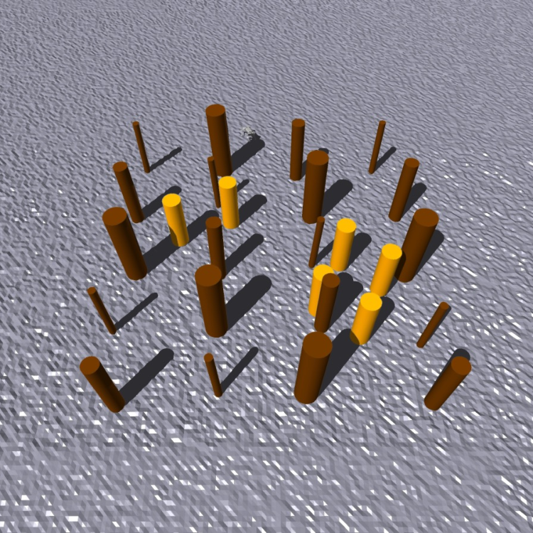
Figure 3: Training environment. (a) Schematic: green start region, pink goal region, central zone with linear-moving dynamic obstacles (yellow cylinders) and static obstacles. (b) A dense realization in Isaac Gym.

An adaptive curriculum over levels $l_c\in\{0,\dots,9\}$ modulates difficulty: the level increments when the robot reaches within 0.5 m of the goal and decrements beyond 2.0 m. Obstacle count scales as $n_o=\lfloor N_o\cdot 0.1\cdot(1+l_c)\rfloor$; the dynamic-velocity envelope expands as $v^{d}_{\max}=\max(v_{\min}^{\text{obj}},0.1(l_c+1)v_{\max}^{\text{obj}})$ with $v^d_{\min}=0.5\,v^d_{\max}$; every 100 steps obstacles may stochastically accelerate or halt with probability $p_{\text{change}}=0.05\,l_c$; and terrain roughness grows linearly from 0 to 7 cm. Training with fast, mostly linear obstacles while evaluating on cooperative RVO crowds is deliberate: RVO agents are expensive to simulate, tend to freeze into congestion that starves the learner of reward, and their conservative deceleration would under-expose the policy to aggressive high-speed interactions.

6. Experiments

The experimental program is organized around three questions: does VOP-Nav raise success rates in crowded dynamic scenes while keeping locomotion fast; does the predicted safe velocity region actually contribute to collision avoidance; and does the policy transfer zero-shot to a physical robot. Five baselines cover the main design families: the classical reciprocal method ORCA (and its derivative variants), the learning-based VO-aided planner NavRL, the crowd-navigation planner HEIGHT, the quadruped crowd-navigation method REASAN, and the agile end-to-end quadruped policy ABS. ORCA and NavRL are additionally evaluated with doubled episode duration (2T) because they are slow walkers whose failures are dominated by timeout rather than collision, and HEIGHT is reported at 4T since its high-level forward-speed command is capped at 0.5 m/s. All newly added legged baselines (ORCA, NavRL, REASAN) share the same REASAN locomotion checkpoint so that differences reflect planning rather than low-level execution.

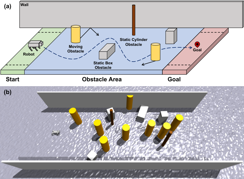
Figure: one of the four unseen test environments (the Forest setting). Dynamic obstacles are yellow cylinders; static trees are brown cylinders in an unstructured, wall-less outdoor layout.

6.1 Main benchmark

Environment	Policy	Success %	Collision %	Timeout %	mean v (m/s)	mean peak v (m/s)
Training	ABS	53.16	43.57	3.26	2.29	3.42
	ORCA(2T)	59.89	22.73	17.38	1.21	2.65
	NavRL(2T)	71.84	22.55	5.61	1.13	2.49
	VOP-Nav	78.35	18.91	2.74	1.99	3.34
Forest	ABS	76.07	23.42	0.50	2.47	3.44
	NavRL(2T)	90.49	8.68	0.84	1.56	2.57
	REASAN	68.06	30.90	1.04	1.67	2.35
	VOP-Nav	94.48	5.42	0.10	2.55	3.56
Office	ABS	61.29	29.33	9.38	2.15	3.35
	NavRL(2T)	81.07	13.60	5.34	1.13	2.52
	VOP-Nav	81.12	14.93	3.95	2.03	3.49
Square	ORCA(2T)	78.79	20.31	0.89	1.50	2.70
	NavRL(2T)	76.37	21.96	1.67	1.22	2.50
	VOP-Nav	83.67	15.67	0.65	1.96	3.35
Slow	ABS	83.92	13.78	2.30	2.30	3.34
	NavRL(2T)	88.89	5.98	5.13	1.09	2.50
	VOP-Nav	92.24	6.08	1.69	2.19	3.42

Selected rows of Table II. Full results include HEIGHT(4T) and REASAN across all five environments; VOP-Nav achieves the highest success rate in every environment.

VOP-Nav attains the best success rate in all five environments, and the margin is largest exactly where the scene is hardest. In the Training environment — restricted space, high obstacle density, and aggressive 1.5 m/s dynamic obstacles — VOP-Nav reaches 78.35% against 71.84% for NavRL(2T), 59.89% for ORCA(2T), 53.16% for ABS, and 43.49% for REASAN, while also moving at 1.99 m/s mean and 3.34 m/s mean peak, speeds no baseline matches. The classical planners ORCA and NavRL buy low collision rates at the cost of enormous timeout rates at standard duration (50.77% and 59.28% respectively); even with doubled time budgets they remain slower and less successful. ABS and REASAN illustrate the opposite failure mode of purely reactive learning: high collision rates of 43.57% and 48.10% in the Training environment. In Forest, VOP-Nav pushes success to 94.48% with only 5.42% collisions and a mean speed of 2.55 m/s, showing that the safety signal does not throttle the robot when the scene allows speed.

The trajectory comparison in the standardized test environment (identical seeds for dynamic obstacles, extra static obstacles to lengthen the route) makes the contrast concrete. HEIGHT collides at step 421 because its slow conservative motion cannot evade a fast obstacle; ORCA enters the crowd at step 270, freezes in a corner for a long period, and finally collides at step 622 when two non-cooperative obstacles eliminate the feasible velocity set; NavRL decelerates sharply at step 270 and squeezes through a gap to finish at step 535, but with dangerously small clearance; REASAN reacts to the first fast obstacle yet fails to brake when several arrive together, colliding at step 278; ABS's recovery policy performs several emergency decelerations but the robot keeps re-entering dense regions and is struck at step 437. VOP-Nav instead decelerates and diverts into open space at steps 146 and 270, accelerates when the path reopens, and reaches the goal at step 437 — earlier than NavRL and with no collision.

Robustness across training seeds was verified by training VOP-Nav with eight seeds. Multi-seed averages track the main checkpoint closely in four of five environments (Training: 77.50% ± 2.05 vs 78.35% for the main checkpoint). Office is the exception with larger variance (success 72.66% ± 6.41, collision 23.60% ± 6.87), attributed to heavy static occlusion limiting observability and amplifying sensitivity to initialization.

6.2 Quality of velocity-obstacle perception

VOP-Net scores IoU 0.808 and MSE 0.172 on validation. Online quality — measured during final policy rollouts by comparing predictions against ground-truth safe regions computed from privileged simulator states — is naturally lower, and is further characterized by the false-safe and false-unsafe rates $\mathrm{FS}=\frac{\sum_j(\ell^{\mathrm{pred}}_j-\ell^{\cap}_j)}{\sum_j\ell^{\mathrm{pred}}_j}$ and $\mathrm{FU}=\frac{\sum_j(\ell^{\mathrm{gt}}_j-\ell^{\cap}_j)}{\sum_j\ell^{\mathrm{gt}}_j}$, which separate over-optimistic errors (declaring unsafe velocities safe) from over-conservative ones (omitting feasible velocities):

Environment	IoU	MSE	FS %	FU %
Training	0.7005	0.2972	16.49	10.21
Forest	0.6883	0.5581	13.28	16.22
Office	0.7792	0.1667	8.52	8.61
Square	0.5520	0.5368	23.92	14.44
Slow	0.7891	0.2309	8.07	10.12

Table IV (VOP-Net rows): online prediction metrics. Square — the densest crowd — yields the lowest IoU and the highest false-safe rate, exactly where perception is hardest.

A GT-VOP-Nav variant, trained with ground-truth safe regions replacing VOP-Net predictions in both input and reward, improves success and substantially reduces collisions in most environments, showing that residual perception errors primarily hurt collision avoidance rather than task completion; Office shows the largest gap because static occlusion challenges onboard prediction. A data-scale study (50%d-VOP-Net trained on half of the 10,000 files) nearly matches full-data validation accuracy (0.806 IoU, 0.174 MSE) but produces higher success-rate variance across seeds, indicating the dataset size mainly buys stability rather than accuracy. Qualitative inspection confirms the network distinguishes approaching threats from receding ones: it partially excludes the future collision region of an approaching obstacle while correctly allowing velocities through the current region of an obstacle that is moving away.

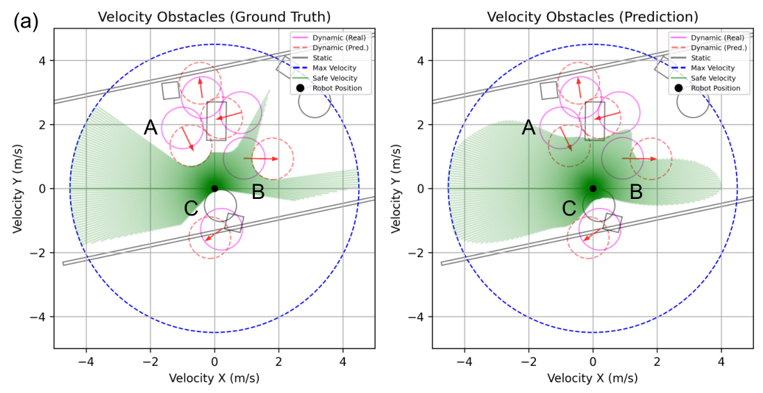
Figure: visualization of safe velocity predictions. Left panel ground truth, right panel VOP-Net prediction; magenta/red circles are current/next-step obstacle positions, green regions are safe velocity sets.

6.3 Ablation: input, reward, or both

Environment	Policy	Success %	Collision %	Timeout %	mean v
Training	Basic	63.76	35.31	0.93	2.14
	Only reward	61.14	27.22	11.64	1.85
	Only input	68.77	30.56	0.67	2.39
	VOP-Nav	78.35	18.91	2.74	1.99
Office	Basic	56.65	42.75	0.60	1.97
	Only reward	36.62	16.66	46.73	1.79
	Only input	72.17	27.24	0.60	2.37
	VOP-Nav	81.12	14.93	3.95	2.03
Square	Basic	66.66	32.79	0.55	2.01
	Only reward	65.42	30.18	4.40	1.80
	Only input	71.52	28.12	0.36	2.41
	VOP-Nav	83.67	15.67	0.65	1.96

Selected rows of Table V. Only input and only reward denote using VOP-Net predictions solely as policy input or solely as reward shaping; VOP-Nav uses both.

The ablation cleanly separates what each integration path contributes. Against the Basic policy, "only reward" lowers collisions but becomes conservative: timeout rates balloon (to 11.64% in Training and 46.73% in Office) and success drops in four environments — a reward signal without perceptual input teaches the robot to hesitate rather than to choose better. "Only input" is the fastest configuration everywhere (mean 2.39–2.50 m/s, peaks up to 4.14 m/s) and beats Basic in all five environments, yet its collision rates stay above VOP-Nav in every environment — safe-velocity information grants agility but not discipline. Combining both yields the best success and collision rates simultaneously: the input tells the policy where safe velocity lives, the reward trains it to respect those bounds. Forest is the one environment where "only reward" matches VOP-Nav, consistent with conservative motion being sufficient in a sparsely constrained scene.

6.4 Real-world deployment

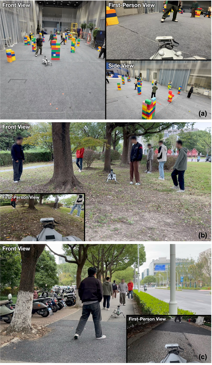
Figure: hardware setup on the Unitree Go2 — Livox Mid-360 LiDAR and RealSense D435i, with compute split across a Jetson Orin Nano and an Intel N100 mini-PC.

Scenario	Trials	Success	Collision	Timeout	peak v (m/s)	mean v (m/s)
Indoor	15	15	0	0	2.462	1.422
Outdoor	15	12	0	1	2.493	1.370

Table VI: real-world results. Indoor trials used motion-capture localization and seven obstructing participants in a 20 m x 8 m area; outdoor trials used Fast-LIO2 in a grove and a 3 m-wide narrow path with eight participants.

The policy trained entirely in simulation deploys zero-shot. Indoor trials achieve 100% success with zero collisions despite participants deliberately stepping into the robot's path. Outdoor trials succeed 12/15: two failures trace to LiDAR-inertial odometry drift accumulated by the robot's aggressive motion, which corrupts the relative-goal and velocity estimates, and one timeout occurred in an extremely narrow passage where the robot chose to wait rather than attempt a risky squeeze. The sim-to-real speed gap (real mean ~1.4 m/s versus ~2 m/s in simulation) is attributed to four factors: human behavior is richer than the linear/stochastic/RVO agents simulated; the Livox Mid-360 is a non-repetitive 60 Hz 3D scanner whose planar extraction leaves empty sectors that are filled with maximum range; localization is noisier outdoors than the motion-capture ideal; and real actuators, latency, foot wear, and uneven terrain reduce executable speed. Stress tests bound the robot's reserves: 3.014 m/s peak speed in open space, an emergency stop for an obstacle thrown 1 m ahead, and stable continuous avoidance against two actively blocking operators without collision or fall.

Three patterns in the numbers repay attention. First, the speed-safety trade-off that dominates every baseline is broken rather than shifted: ORCA-family planners reduce collisions only by walking slowly and timing out, ABS and REASAN move fast but collide in roughly a third to half of Training episodes, whereas VOP-Nav improves both axes simultaneously relative to the Basic policy (success +14.59 points, collisions -16.40 points in Training). This is precisely what the dual-use design predicts: the input expands the set of velocities the policy dares to use, while the reward removes the unsafe part of that set. Second, VOP-Nav's mean velocity of successful trajectories (1.96-2.55 m/s across environments) is nearly twice that of ORCA and NavRL variants and approaches ABS's 2.15-2.47 m/s, yet ABS achieves those speeds with collision rates 1.3-2.9x higher. Third, the environments where VOP-Net's online prediction quality is highest (Office IoU 0.7792, Slow 0.7891) coincide with its largest success margins over reactive baselines, while Square - the densest crowd with the worst perception (IoU 0.5520, FS 23.92%) - is where the residual gap to a ground-truth oracle remains most visible. The data-scale study adds a practical engineering conclusion: the 10,000-file dataset (1,024 environments x 48 steps each) is not excessive; halving it preserves mean accuracy but measurably destabilizes training across seeds, so the dataset acts as a variance reducer for downstream policy learning.

One more implementation detail deserves attention because it explains why the whole system fits on cheap embedded hardware. The perception network is deliberately lightweight — MobileNet blocks over a compact three-channel tensor plus two orthogonal attention pools — and it runs at 50 Hz on a Jetson Orin Nano 8GB, while the 1693-dimensional policy runs on a separate Intel N100 mini-PC. Neither module requires a GPU-class workstation at deployment time, and the low-level PD controller at 200 Hz closes the loop on joint targets. This split makes VOP-Nav practical for production quadruped platforms where compute and power budgets are tight, in contrast to approaches that depend on heavy dense point-cloud backbones or large transformer planners. It also isolates failure modes: if VOP-Net degrades, the policy still receives its full proprioceptive and depth input, and the reward-shaped training means the policy has internalized part of the safety behavior rather than blindly copying the perception output.

7. Limitations

Two limitations are stated by the authors. First, VOP-Net operates on a 2D planar representation; this ignores the 3D traversability that is the whole point of a legged platform — overhanging structures and negative obstacles such as ditches require volumetric perception that a planar safe-velocity map cannot provide. Second, outdoor robustness is bounded by LiDAR-inertial odometry drift under aggressive motion, which directly caused two of the three outdoor failures. Beyond the authors' list, two more deserve emphasis. The perception stack assumes a specific LiDAR configuration: empty angular sectors from the non-repetitive scan pattern are patched with maximum-range values, a heuristic that could mislead the policy when real occlusion patterns differ from training-time ray casting. And the training-time obstacle model — cylinders and cuboids on linear or mildly stochastic trajectories — is a substantial simplification of pedestrian dynamics; the RVO-based evaluation crowds are a step toward realism, but genuine human intentions, groups, and social conventions remain outside the training distribution, as the reduced real-world speeds confirm.

8. Conclusion and Outlook

VOP-Nav resolves the classic tension between geometric safety and learned agility by moving the velocity-obstacle computation out of the fragile detection-and-tracking pipeline and into a learned perception module. VOP-Net turns five frames of raw LiDAR into a 360-direction safe-velocity map, and that map is used twice: as policy input at inference and as reward shaping at training. The result is a single end-to-end system that leads every simulated benchmark in success rate while remaining the fastest successful policy, and that transfers zero-shot to a Unitree Go2 with commodity sensors and split embedded compute. The natural next steps follow directly from the stated limitations: lifting the safe-velocity representation into 3D traversability, tightening outdoor localization, and closing the remaining perception gap on the hardest crowds (Square's 0.552 online IoU shows where the headroom is). The broader lesson is methodological: classical safety geometry and end-to-end learning compose best when the geometry is expressed as a learnable signal rather than enforced as a hard constraint.

9. Golden Quote

"The input provides safe velocity information, while the reward regulates its use, yielding the strongest overall balance between progress and safety."

This deep read is based on the full text of arXiv:2607.15036v1.