Memory for Attention: Language-Conditioned Re-Perception with a Vision--Language--Motion Map

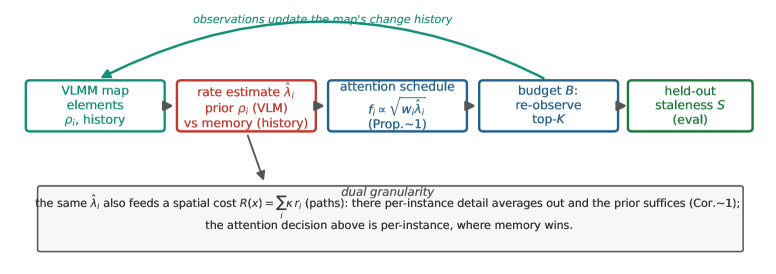
Figure 1 — Budgeted re-perception as attention. The map holds each element's change history; a rate estimate $\hat{\lambda}_i$ is formed from the on-demand category prior (VLM) or the map's observed history (memory). The $\sqrt{\cdot}$-law schedule sets re-check frequencies.

1. Background & Motivation

A robot carrying a persistent behavior-annotated map (e.g., Vision–Language–Motion Maps, VLMM) faces two very different planning questions, and its memory answers only one well.

• Spatial navigation: how to walk around a room? A behavior-aware planner cost cuts a planning-time objective by ~35% over 28 AI2-THOR scenes, but under closed-loop execution the real benefit nearly vanishes (~4%), and an on-demand VLM does as well.
• Resource allocation: under a limited perception budget, what should the robot attend to right now to keep its map fresh? Framing re-perception as this attention decision — which map elements to re-observe, and how often — a persistent map's memory yields the best re-perception schedule.

The map earns its keep not by telling the robot how to walk around a room, but by telling it what to pay attention to.

2. Core Methodology

2.1 The Attention Decision

The map holds $N$ elements. Element $i$ changes as a Poisson process of rate $\lambda_i$; if re-observed every $\tau_i$ steps, its time-average staleness is:

$$g(\lambda_i \tau_i) = 1 - \frac{1 - e^{-\lambda_i \tau_i}}{\lambda_i \tau_i} \approx \frac{1}{2} \lambda_i \tau_i, \quad \lambda_i \tau_i \ll 1$$

Element $i$ carries importance $w_i$. Under a perception budget of $K$ re-observations per step, the attention policy chooses $f_i = 1/\tau_i$ with $\sum_i f_i = K$ to minimize $S = \sum_i w_i\, g(\lambda_i \tau_i)$.

2.2 Proposition 1: $\sqrt{\cdot}$-Law Attention

Minimizing $S \approx \sum_i w_i \lambda_i / (2f_i)$ s.t. $\sum_i f_i = K$ yields the optimal frequency:

$$f_i^\star \propto \sqrt{w_i \lambda_i}, \quad S^\star = \frac{\left(\sum_i \sqrt{w_i \lambda_i}\right)^2}{2K}$$

Re-check frequency is proportional to the geometric mean of importance and change rate.

2.3 Proposition 2: Attention Loss from Rate Error

With estimate $\hat{\lambda}_i$, the realized cost is $S(\hat{\lambda}) = \frac{1}{2K}(\sum_i a_i)(\sum_i b_i^2 / a_i)$ where $a_i = \sqrt{w_i \hat{\lambda}_i}$, $b_i = \sqrt{w_i \lambda_i}$. The excess is a Cauchy–Schwarz defect growing as $\hat{\lambda}$ diverges from $\lambda$.

2.4 Corollary 1: Freshness Gap = Root-Volatility Variance

For uniform importance, a memoryless uniform baseline incurs $\propto \mathbb{E}[\lambda]$, while the $\sqrt{\cdot}$-law optimum incurs $\propto (\mathbb{E}\sqrt{\lambda})^2$. Their gap is exactly:

$$\mathrm{Error}_{\mathrm{VLM}} - \mathrm{Error}_{\mathrm{Map}} \propto \mathbb{E}[\lambda] - (\mathbb{E}\sqrt{\lambda})^2 = \mathrm{Var}\!\left(\sqrt{\lambda}\right) \geq 0$$

The value of memory equals the heterogeneity of the scene's dynamics, measured as $\mathrm{Var}(\sqrt{\lambda})$. It vanishes when all instances share a rate and grows linearly with spread.

2.5 Rate Estimate Sources

• On-demand VLM: returns category movability prior $\rho_i$ — one value per object type.
• Map memory: accumulates per-element change history into a Bayesian rate $\hat{\lambda}_i = (m_i + \kappa\rho_i)/(t_i + \kappa)$, with $m_i$ observed changes over $t_i$ time.

2.6 Heterogeneity Knob

Modeled with $h \in [0,1]$: $\lambda_i = \lambda_{\max}[(1-h)\rho_i + h\, u_i]$, $u_i \sim \mathrm{U}(0,1)$. At $h=0$ every instance equals its category prior (memory adds nothing); at $h=1$ instance rates are independent of category (only history can know them).

flowchart TD
    MAP["Persistent map\nN elements + change history"] --> EST["Rate estimate λ̂_i"]
    VLM["On-demand VLM\ncategory prior ρ_i"] --> EST
    EST -->|"√-law schedule\nf_i ∝ √(w_i·λ̂_i)"| SCHED["Re-check schedule\nbudget K"]
    SCHED --> REOBS["Re-observe K elements"]
    REOBS -->|"Update history"| MAP
    SCHED --> SCORE["Score: value-weighted staleness S"]
    EST -.->|"Spatial cost (path planning)\ndetail averages out, prior suffices"| SPATIAL["Path planning\n(no memory advantage)"]
    EST -.->|"Attention decision (per-instance)\nmemory wins"| ATT["Resource-allocation attention\n(memory advantage)"]
    style MAP fill:#dbeafe,stroke:#2563eb
    style VLM fill:#fed7aa,stroke:#ea580c
    style SCHED fill:#dcfce7,stroke:#16a34a
    style ATT fill:#fef3c7,stroke:#d97706

Figure M1 — Attention decision framework. The map's change history or VLM category prior forms a rate estimate; the $\sqrt{\cdot}$-law schedule sets re-check frequencies. Dual granularity: the same estimate feeds path planning spatial cost (detail averages out, prior suffices), but the attention decision is per-instance where memory wins.

3. Experimental Results

In AI2-THOR, 951 movable object instances pooled from 40 scenes. Parameters: $\lambda_{\max}=0.12$, horizon $T=400$, budget $K=6\%$ per step. Held-out estimate: change history accumulated on one realization, frozen, applied as static schedule to an independent realization.

3.1 Memory Beats On-Demand Prior

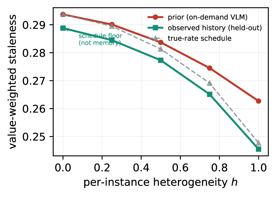
Figure 2 — As heterogeneity increases, held-out history lowers value-weighted staleness below the on-demand prior.

Heterogeneity $h$	0	0.25	0.5	0.75	1.0
Prior (VLM)	.294	.290	.284	.275	.263
Memory (history)	.289	.285	.277	.265	.246
Advantage (%)	1.7	1.9	2.3	3.4	6.5
Memory-attributable (%)	0.0	0.2	0.6	1.7	4.9

3.2 Against Competitive Schedulers: The Prior Is the Weak Link

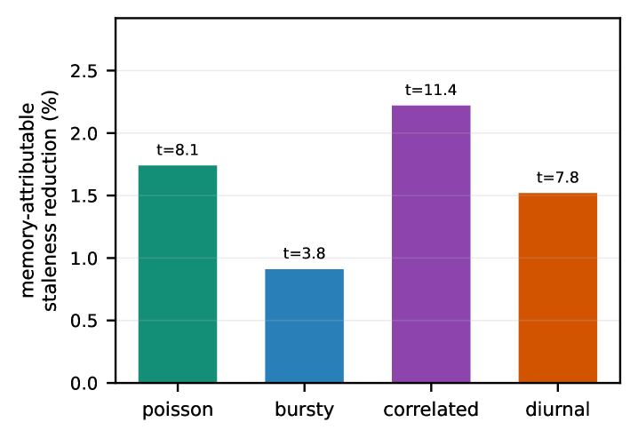
Figure 3 — Competitive schedulers, run online (skewed importance). The on-demand VLM prior is beaten even by memory-light oldest-first; history-based policies win and memory matches the oracle.

Adding competitive schedulers reveals: (1) the on-demand VLM prior is the weak link — even memory-light oldest-first beats it at every $h$; (2) history-based policies win: Thompson tracks memory, and memory matches the oracle (0.248 vs 0.248 at $h=1$).

3.3 Whittle Index Removes the Schedule Floor

Budgeted re-perception is a restless multi-armed bandit; the Whittle index is closed-form:

$$W_i(\tau) = w_i\left[\frac{1 - (1-\lambda_i)^\tau}{\lambda_i} - \tau(1-\lambda_i)^\tau\right]$$

The Whittle policy beats the $\sqrt{\cdot}$-law (4.1% lower staleness with true rates). Under the proper index, memory beats the prior only where heterogeneity is real ($-1.2\%$ at $h=0$ rising to $+4.5\%$ at $h=1$), with no floor to subtract.

Heterogeneity $h$	0	0.25	0.5	0.75	1.0
Whittle prior	.282	.278	.271	.259	.237
Whittle memory	.285	.282	.275	.264	.243
Memory vs prior (%)	-1.2	-0.9	-0.3	+0.9	+4.5

3.4 Language-Conditioned Task: Distinctive Value

When the task is language-conditioned, VLMM grounds relevant objects (open-vocabulary) and tracks their change (memory), beating strong baselines: +2.5% vs relevance-weighted recency, +8.9% vs on-demand VLM. The motion channel adds value beyond a last-seen timestamp.

4. Contributions & Significance

• Distinguishes two uses of behavior-annotated maps: spatial-navigation path-shaping (marginal under closed-loop, no memory needed) vs. resource-allocation attention (memory pays off).
• Formalizes budgeted re-perception as an attention decision, deriving the $\sqrt{\cdot}$-law optimal schedule.
• Proves the memory-vs-prior freshness gap equals $\mathrm{Var}(\sqrt{\lambda})$ — root-volatility variance — growing linearly with scene heterogeneity.
• Introduces the Whittle index scheduler to remove the $\sqrt{\cdot}$-law heuristic floor, cleanly isolating memory-attributable gains.
• Shows VLMM's motion channel exceeds last-seen timestamps in language-conditioned tasks.

5.

模糊核函数

$$ g(\lambda_{i}\tau_{i})=1-\tfrac{1-e^{-\lambda_{i}\tau_{i}}}{\lambda_{i}\tau_{i}}\approx\tfrac{1}{2}\lambda_{i}\tau_{i} $$

Limitations

• The $\sqrt{\cdot}$-law is optimal for the continuous surrogate, not the exact discrete budgeted optimum.
• The memoryless VLM baseline models a VLM returning the category mean; a real VLM may do better or worse.
• Established under Poisson processes; robust under alternatives (bursty, correlated, diurnal) but attenuated under burstiness.

6. Conclusion

This paper distinguishes two planning uses of a behavior-annotated map. In spatial navigation, the benefit of behavior-aware path shaping nearly vanishes under closed-loop execution (~4%), and an on-demand VLM is equally effective — map memory is useless here. But in resource-allocation attention, the memory's change history yields a re-perception schedule matching an oracle, while the on-demand VLM prior is a poor scheduler. The memory-vs-prior freshness gap equals exactly $\mathrm{Var}(\sqrt{\lambda})$, growing linearly with scene heterogeneity. In language-conditioned tasks, VLMM's open-vocabulary grounding and change tracking surpass last-seen timestamps and on-demand VLMs. The map earns its keep not by telling the robot how to walk around a room, but by telling it what to pay attention to — memory justifies its existence in attention allocation.