PAPER DEEP DIVE
HAM-VLN: Harnessing Hierarchical Agentic Memory for Zero-Shot Vision-and-Language Navigation
Vision-and-language navigation (VLN) enables robots to follow instructions in previously unseen environments. Recently, a training-free paradigm has emerged: the robot queries a multimodal LLM to understand its observations and plan the next action. However, long-horizon navigation based on either image streams or dense map inevitably introduces a growing memory and reasoning bottleneck. We present HAM-VLN, a decision-coupled, agent-authored memory that equips the robot with a persistent, depth-grounded world graph. In the same model call used to select the next action, HAM-VLN also records semantic and reflective information—including room type, objects, navigation progress, and failure notes. Recent waypoints remain verbatim within a bounded window, while older history re-enters the context only through retrieval scored by relevance, recency, and salience, together with one-hop topological expansion. This design requires no additional LLM calls beyond the per-waypoint decision. Compared to previous methods, HAM-VLN not only improves various navigation metrics but also reduces the context length by more than 65%. Specifically, HAM-VLN achieves 61.0% Success Rate (SR) on VLN-CE R2R, 52.7% SR on VLN-CE RxR, and 79.7% SR on HM3D-v2 ObjectNav without any training.
TL;DR
HAM-VLN makes the single planning call it already has to pay for double as a memory writer: the same Gemini invocation that chooses a direction also records room type, observed objects, instruction progress, and the reason for a failure into a world graph built by depth back-projection. Old history only returns to context when the current subgoal retrieves it. With no training and no extra model calls, it reaches 61.0% success rate on VLN-CE R2R, 52.7% on RxR, and 79.7% on HM3D-v2 ObjectNav, while compressing per-episode context by 67%.
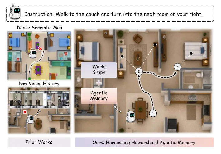
Figure 1: Prior systems (left) present navigation history either as a dense semantic map, whose storage grows with mapped area, or as raw visual history, whose context grows with the trajectory. HAM-VLN (right) stores long-term history in a depth-grounded world graph and uses hierarchical agentic memory to decide what stays in context and what is retrieved per decision.
Background: In Zero-Shot VLN the Bottleneck Is Memory, Not the Model
Vision-and-language navigation asks a robot to follow a natural-language instruction to a goal location or goal object in an environment it has never seen. Multimodal large language models made "navigate without training" possible: at each waypoint the robot hands its current observation to the model, which interprets the scene and picks the next action. The appeal of this zero-shot regime is that it decouples navigation competence from "how many trajectories can I supervise" and reattaches it to "how much common sense does the pretrained model hold".
But any single model call can only reason over what that call sees. As trajectories grow long, later decisions depend on three things that are not in the current image: which places the robot has already visited, how far the instruction has been executed, and which branch has already been tried and failed. Feeding those facts to the model without letting context grow without bound is what this paper calls the memory bottleneck.
The paper sorts existing designs into two families and names how each one fails. The first is the dense semantic map: tensors aligned to pixels or voxels, whether closed-category labels or open-vocabulary features. Storage grows with mapped area, and, more damaging, the contents are built separately from the navigation decision, so instruction fragments such as "the table in the bedroom" or "the hallway toward the kitchen" must then be matched back onto metric grid cells. Semantics and geometry sit on either side of a mapping layer. The second family is raw visual history: past panoramas appended to the model context. Landmarks get buried among other visual details, context grows at every step, and a dead end that was already walked is never marked as a branch to avoid.
The diagnosis is sharp and worth quoting in substance: both representations make past observations available, but the MLLM never decides what to retain for later decisions. History is accumulated passively rather than authored by the agent.
A second thread comes from LLM agent memory research. Generative Agents organize a memory stream by relevance, recency, and importance, and reflect over accumulated experience; MemGPT manages a bounded model context through external memory; Reflexion keeps verbal feedback from unsuccessful attempts to guide later behavior. Embodied navigation adds a spatial requirement to all of this: a useful memory must preserve where objects were observed, how visited regions connect, how far the instruction has progressed, and where previous decisions failed. HAM-VLN positions itself as the coupling of Generative-Agents-style memory principles to a robot's spatial experience and its current subgoal.
Preliminaries: Waypoints, the Four Metrics, and the Dual-Process Split
Reading the numbers requires separating two granularities. The low-level action $A_t \in \mathcal{A}_{\mathrm{robot}}$ is an executable action in a continuous environment (advance a short distance, turn a small angle), while a decision waypoint is a pose where the robot stops, looks around, and makes one high-level decision. The MLLM is invoked only at waypoints; between waypoints a deterministic controller executes continuously. All token costs in the paper therefore come in two scales: per decision and per episode.
On metrics: NE (navigation error) is the straight-line distance from the stopping point to the goal, lower is better; SR is success rate; OSR is oracle success rate, counting an episode as successful if the trajectory ever entered the success region; SPL weights success by the ratio of shortest to executed path length and therefore measures efficiency; RxR, whose instructions are longer, additionally reports nDTW (normalized dynamic time warping) as a measure of alignment with the reference path. A high SR with a low SPL usually means "found it, but took the long way round", and that combination recurs throughout the ablations below.
Architecturally, HAM-VLN follows hierarchical VLA and dual-system VLN designs: a slow, deliberative System 2 decides where to go and why, while a fast, reactive System 1 grounds that intent in the pixel space of the current observation and converts it into executable motion. The split is simultaneously a compute split. Expensive reasoning happens once per waypoint; the perception-to-action loop is carried by a lightweight model plus a geometric controller.
Method
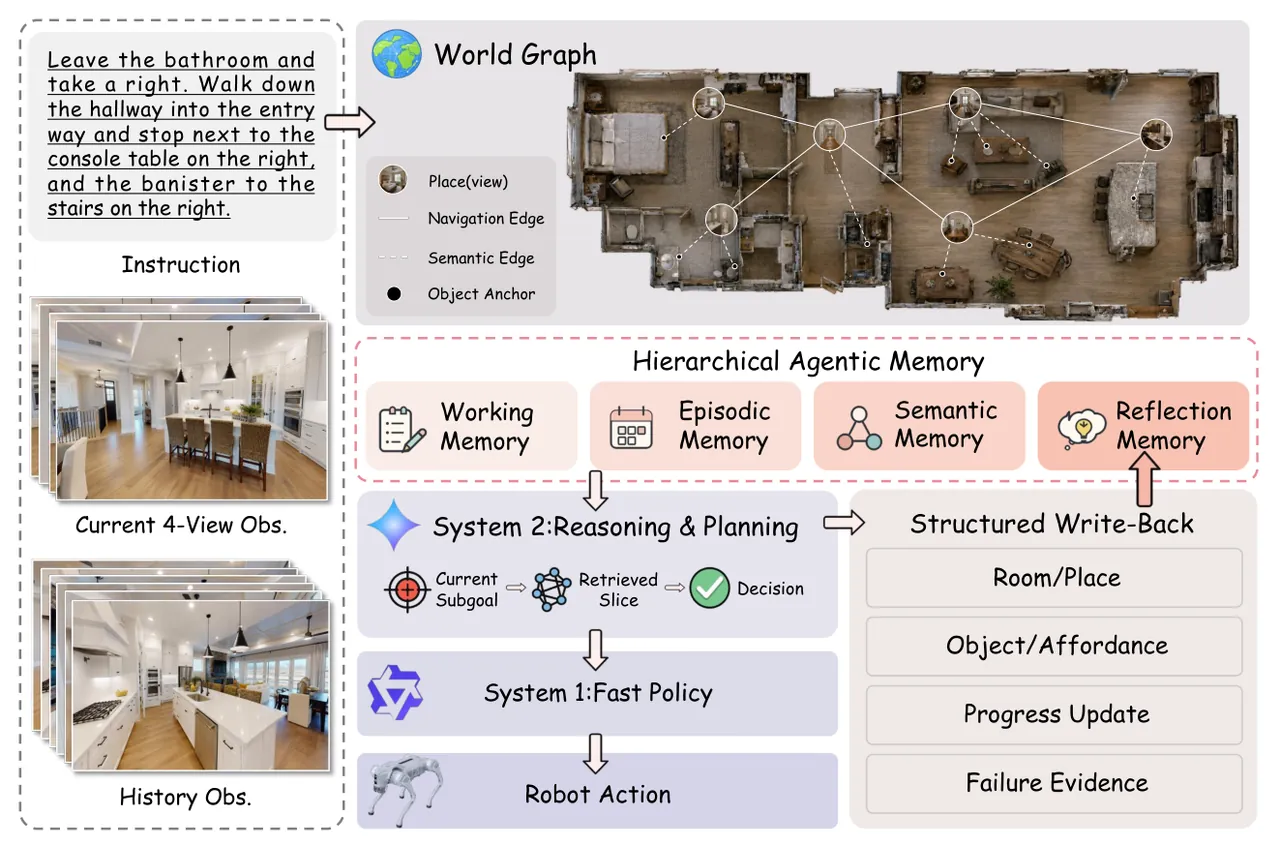
Figure 2: Overview. At each waypoint System 2 reads the current panorama, a bounded working memory of $K$ waypoint transitions, and a retrieved graph slice, then returns both the navigation action and the memory writes (room type, objects, progress, failure note) inside one structured call. System 1 grounds the chosen direction to pixels and the controller executes it. The task-relevant slice retrieved for the current subgoal re-enters the context of the next planning call.
1. Dual-process architecture: one call does two jobs
The full-step policy is decomposed into a composite map:
$$A_{t}=\pi_{\mathrm{robot}}\big(\varphi_{1}\big(\varphi_{2}(\mathcal{T},O_{t},M_{t})\big),\,D_{t},P_{t},\mathbf{K}_{\mathrm{cam}}\big)$$
where $\mathcal{T}$ is the instruction, $O_t$ the observation at the current waypoint, $M_t$ the retrieved memory context, $D_t$ the corresponding depth observation, $P_t$ the odometry pose, and $\mathbf{K}_{\mathrm{cam}}$ the camera intrinsics. The paper uses lowercase $a_t$ for the high-level decision produced by System 2 to keep it distinct from the low-level action $A_t$ in the simulator's action space.
System 2 (reasoning and planning) is $\varphi_2$, a large MLLM invoked once per waypoint, that is, at the pose where the robot stops, looks around, and decides. Reading $\mathcal{T}$, $O_t$, and $M_t$, it commits to one discrete decision: pursue a direction, backtrack to a previously visited waypoint, or stop after verification. The point of the design is that this decision arrives wrapped in a structured JSON record that also carries progress analysis and action reasoning. Writing memory is not an extra call; it is a byproduct of the call that was already being paid for.
System 1 (fast policy) is $\varphi_1$, a lightweight grounding-specialized MLLM. It observes the selected view together with the planner's target description and predicts the target bounding box directly, with no pretrained waypoint predictor. The authors stress this because it preserves the ability to ground distant semantic cues: a goal such as "the hallway opening" rarely corresponds to any explicit intermediate waypoint. The deterministic controller $\pi_{\mathrm{robot}}$ then picks a representative pixel inside the predicted box, back-projects it to 3D using the depth map and intrinsics, transforms it into world coordinates with the odometry pose, and runs fast-marching planning on a lightweight local traversability map to execute a short-horizon trajectory.
2. Memory state: working memory, progress record, world graph
At decision waypoint $t$, $W_t$ is the frame stream retained from the most recent $K$ completed waypoint transitions, $L_t$ is the ordered instruction-progress record, and $G_t$ is the long-term world graph accumulated over the episode. The current subgoal $q_t$ is derived from $L_t$ (its first incomplete item), and the memory context handed to System 2 is
$$M_{t}=W_{t}\oplus L_{t}\oplus\mathcal{R}(G_{t},q_{t})$$
$\mathcal{R}$ is a query-conditioned read operator and $\oplus$ denotes assembly into the planning context; the current panorama $O_t$ is immediate perception and is supplied separately rather than charged to the memory budget. The definition of $K$ is what makes this a hard boundary: inside the window, visual history is kept verbatim; outside it, old observations can only return through a structured readout of $G_t$. Every experiment in the paper uses $K{=}1$, so verbatim retention covers exactly the frames of the last transition.
Long-term state is a typed place-object graph:
$$G_{t}=\big(\mathcal{V}^{P}_{t},\ \mathcal{V}^{O}_{t},\ \mathcal{E}^{PP}_{t},\ \mathcal{E}^{PO}_{t}\big)$$
Place nodes $\mathcal{V}^P_t$ are formed by incremental single-link clustering; each place state aggregates spatial anchors, agent-authored semantic context, visitation statistics, and optional failure evidence. Object nodes $\mathcal{V}^O_t$ associate one depth-grounded category observation with open-vocabulary descriptions and soft attributes at the place/category level. Place-place edges $\mathcal{E}^{PP}_t$ encode navigational connectivity and place-object edges $\mathcal{E}^{PO}_t$ encode semantic containment together with its confidence.
The difference from a dense semantic map lies in the independent variable of growth: this graph grows with the places and entities the robot discovers, not with the area mapped, while still retaining the geometry and topology needed for recall and backtracking. That is the substance of the paper's first contribution.
3. Decision-coupled updates: what the agent writes, what is automatic
A System 2 call produces one structured decision record $J_{t}=(a_{t},w_{t},r_{t})$: $a_t$ is the high-level action, $w_t$ carries place semantics, observed objects, and instruction-progress updates, and $r_t$ is the action rationale. Let $\Gamma(O_t,D_t,P_t)$ denote the anchored geometric evidence extracted from the current RGB-D observation and pose. Progress state and world model then evolve jointly:
$$L_{t+1}=\mathcal{U}_{L}(L_{t},w_{t}),\qquad G_{t+1}=\mathcal{U}_{G}\!\left(G_{t},w_{t},\Gamma(O_{t},D_{t},P_{t})\right)$$
$\mathcal{U}_L$ applies the progress update; $\mathcal{U}_G$ associates observations with places and objects, merges duplicate evidence, and updates topology. When $a_t$ is a backtrack, the event-specific update of Section 3.4 attaches $r_t$ as failure evidence. The division of labor is explicit and clean: $w_t$ and $r_t$ are authored by the agent, while grounding, association, projection, and graph maintenance are automatic. Open-set detection and segmentation come from Grounding DINO and SAM, and their outputs are merged into place-level object states after depth projection.
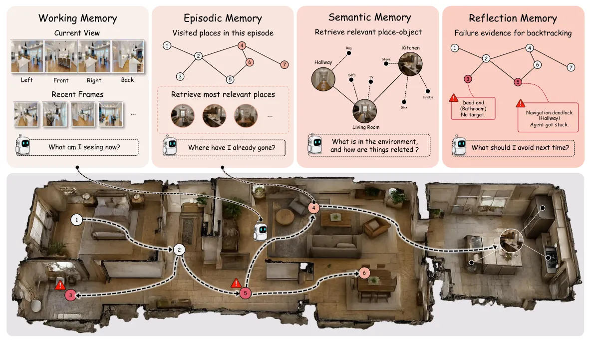
Figure 3: Four functional memory views over one episode. (1) Working memory: the recent egocentric frame stream inside the $K$-waypoint window, the part the planner sees verbatim. (2) Episodic memory: temporal retrieval over visited places, supplying recency. (3) Semantic memory: content retrieval over the place-object graph, supplying relevance. (4) Reflection memory: notes attached to abandoned places, resurfacing verbatim when that place is retrieved.
The paper is careful that these are not four separate stores but four read patterns over the same state in equation (2): episodic memory reads visitation traces and time metadata in $G_t$ (recency), semantic memory reads place-object content and topology (relevance), and reflection memory returns the failure evidence attached to whichever place got retrieved. Salience in the retrieval score is an importance term derived from landmark and object evidence; reflection is orthogonal to scoring and re-enters context only when its place is retrieved.
4. Subgoal-conditioned retrieval: three-term scoring and one-hop expansion
At waypoint $t$ the first open item of $L_t$ defines the current subgoal $q_t$. A local sentence encoder (bge-large-en-v1.5, resident on each worker GPU) embeds $q_t$ and the summary of every place state $p\in\mathcal{V}^P_t$ into one space, then scores with a weighted sum of three terms:
$$s_{t}(p)=\alpha\,\mathrm{rel}(q_{t},p)+\beta\,\mathrm{rec}_{t}(p)+\gamma\,\mathrm{sal}(p)$$
$\mathrm{rel}$ is cosine similarity between query and place, $\mathrm{rec}_t(p)=\rho^{\,t-\tau(p)}$ decays exponentially from the most recent visit $\tau(p)$, and $\mathrm{sal}$ combines landmark agreement and object richness. All experiments fix $(\alpha,\beta,\gamma)=(1.0,0.3,0.3)$ with a per-waypoint decay $\rho=0.85$, so relevance dominates while recency and salience each carry roughly a third of that weight. The three terms correspond to task relevance, temporal continuity, and perceptual importance.
The read operator $\mathcal{R}(G_t,q_t)$ is not a plain top-$k$. With a seed budget $K_s=3$ it takes the three highest-scoring places as seeds, expands them by one hop, includes the current place's neighborhood, and keeps at most $K_p=5$ places. The resulting place-object subgraph is serialized into $M_t$ together with semantic content, relative geometry, topology, and any associated failure evidence. This is where topology awareness pays off: the decision a navigator needs is often not the room most similar in embedding space but the corridor next to it and how the two connect.
5. Grounded failure memory: backtracking as a coupled control-memory transition
Under partial observability, an abandoned branch is not merely motion to be undone; it is negative evidence about whether the current subgoal is compatible with a region already explored. So when System 2 decides to return to a previously visited waypoint $b_t$, the abandoned suffix $\mathcal{B}_t$ is mapped onto its associated place states and the rationale $r_t$ is stored as grounded failure evidence. The algorithm writes this as
$$\mathcal{F}_{t}\leftarrow\mathrm{Places}(\mathcal{B}_{t})\setminus\{p(b_{t})\},\qquad G_{t+1}\leftarrow\mathrm{MarkFailure}(G_{t+1},\mathcal{F}_{t},r_{t})$$
One distinction is easy to miss but design-critical: the return target is waypoint-level (to preserve executable geometry) while the evidence is place-level (so it survives repeated visits).
This evidence is advisory rather than prohibitive: it neither changes $s_t(p)$ nor blocks any place. It re-enters $M_t$ only when $\mathcal{R}(G_t,q_t)$ retrieves the associated region, letting System 2 reinterpret the earlier failure under the current subgoal. Backtracking therefore changes both the agent's pose and the memory state on which later decisions are conditioned, closing the loop from action and failure, to grounded write, to conditional recall, to revised action.
Algorithm 1 strings the episode together: initialize $L_0$ from the instruction $\mathcal{T}$ and empty $G_0, W_0$; at each waypoint receive $(O_t,D_t,P_t)$, derive $q_t$, assemble $M_t$, call $\varphi_2$ for $(a_t,w_t,r_t)$, and update $L$ and $G$; if $a_t$ is Stop, return; if it is Backtrack, mark failure and return to anchor $b_t$; otherwise $\varphi_1$ produces the target $g_t$ for the controller to execute. Finally $\mathrm{UpdateWindow}(W_t,O_t;K)$ rolls the working-memory window forward.
flowchart TD
  OBS["Waypoint observation<br/>panorama O_t + depth D_t + pose P_t"] --> SUB["Take first incomplete item of L_t<br/>to form subgoal q_t"]
  SUB --> READ["Read operator R(G_t, q_t)<br/>local bge embeddings score s_t(p)<br/>K_s=3 seeds + one hop + K_p=5"]
  WM["Working memory W_t<br/>frames of last K transitions, K=1"] --> CTX["Assemble context<br/>M_t = W_t + L_t + R(G_t, q_t)"]
  READ --> CTX
  CTX --> S2["System 2: Gemini-3.1-Pro<br/>one call returns JSON<br/>J_t = (a_t, w_t, r_t)"]
  S2 --> WL["U_L updates instruction progress L_t+1"]
  S2 --> WG["U_G updates world graph G_t+1<br/>Grounding DINO + SAM + depth back-projection"]
  S2 --> BR{"Which kind of action is a_t?"}
  BR -->|"direction"| S1["System 1: Qwen3.6-35B<br/>predicts target bbox"]
  S1 --> CTRL["Controller: pick pixel in bbox<br/>back-project to world frame<br/>fast marching local plan"]
  BR -->|"backtrack to b_t"| FAIL["MarkFailure<br/>attach r_t to places of abandoned suffix"]
  FAIL --> CTRL
  BR -->|"verified stop"| DONE["episode ends"]
  CTRL --> WM
Experiments
Main results: the first training-free system to lead on all four metrics
On R2R-CE val-unseen, HAM-VLN improves over the strongest prior training-free baseline across the board: NE drops from 5.87 m to 3.92 m, while OSR, SR, and SPL rise by 27.7, 22.7, and 19.0 percentage points. On RxR-CE, whose instructions are longer and harder to align, the same configuration lowers NE from 8.80 m to 6.27 m and raises SR, SPL, and nDTW by 18.9, 19.6, and 8.6 percentage points, and the authors emphasize that this comes without benchmark-specific retuning.
| Method | Type | R2R NE ↓ | R2R OSR ↑ | R2R SR ↑ | R2R SPL ↑ | RxR NE ↓ | RxR SR ↑ | RxR SPL ↑ | RxR nDTW ↑ |
|---|---|---|---|---|---|---|---|---|---|
| NaVILA | supervised | 5.22 | 62.5 | 54.0 | 49.0 | 6.77 | 49.3 | 44.0 | 58.8 |
| StreamVLN | supervised | 4.98 | 64.2 | 56.9 | 51.9 | 6.22 | 52.9 | 46.0 | 61.9 |
| JanusVLN | supervised | 4.78 | 65.2 | 60.5 | 56.8 | 6.06 | 56.2 | 47.5 | 62.1 |
| OmniNav | supervised | 3.74 | 74.6 | 69.5 | 66.1 | 3.77 | 73.6 | 62.0 | -- |
| SPAN-Nav | supervised | 4.07 | 75.3 | 66.3 | 59.3 | 4.20 | 69.7 | 60.1 | 67.9 |
| InstructNav | training-free | 6.89 | 47.0 | 31.0 | 24.0 | -- | -- | -- | -- |
| GC-VLN | training-free | 7.30 | 41.8 | 33.6 | 16.3 | 8.80 | 33.8 | 13.8 | -- |
| LaViRA | training-free | 6.54 ±0.27 | 48.7 ±2.1 | 38.3 ±0.6 | 28.3 ±0.9 | -- | -- | -- | -- |
| Three-Step Nav | training-free | 5.87 | 39.0 | 34.0 | 29.1 | 9.21 | 22.0 | 16.1 | 45.7 |
| HiMemVLN | training-free | 6.65 | 36.0 | 30.0 | 26.9 | -- | -- | -- | -- |
| HAM-VLN (ours) | training-free | 3.92 ±0.15 | 78.7 ±3.1 | 61.0 ±1.7 | 48.1 ±0.2 | 6.27 ±0.23 | 52.7 ±1.5 | 35.7 ±2.6 | 54.3 ±0.3 |
Table 1 (excerpt of the paper's Table 1): main results on VLN-CE R2R and RxR val-unseen. Our numbers are mean ± standard deviation over three seeds; the remaining entries are as reported by their respective papers.
Two caveats deserve to be stated by the reader rather than by the abstract. First, HAM-VLN's OSR on R2R (78.7) already exceeds every supervised method in the table, yet the strongest trained systems still hold higher SR and SPL. The authors' own explanation is that agentic exploration samples the next direction under uncertainty, whereas a learned policy walks "learned shortcuts". The OSR-to-SR gap (78.7 versus 61.0) is that difference quantified: the robot frequently passes the correct location without stopping. Second, evaluation uses 100-episode subsets rather than the full val-unseen split. The paper cites Ding et al. to argue that subset SR differs from the full split by no more than 1.1 percentage points, but that is still a discount to keep in mind.
On HM3D-v2 ObjectNav, HAM-VLN reaches SR 79.7 ±0.5 and SPL 43.2 ±0.6, which is 3.5 and 4.5 points above the best prior training-free result and also above the best supervised result in the table (FiLM-Nav, 77.0 / 41.3) by 2.7 and 1.9 points. The attribution is room-level semantic priors acquired during MLLM pretraining: goal-room associations such as "find a bed in the bedroom" come free in the zero-shot route, whereas the supervised route must have them covered by data.
| Method | Type | SR ↑ | SPL ↑ |
|---|---|---|---|
| DD-PPO | supervised | 27.9 | 14.2 |
| PIRLNav | supervised | 70.4 | 34.1 |
| Uni-NaVid | supervised | 73.7 | 37.1 |
| FiLM-Nav | supervised | 77.0 | 41.3 |
| VLFM | training-free | 62.6 | 31.0 |
| ApexNav | training-free | 76.2 | 38.0 |
| DSCD-Nav | training-free | 73.0 | 38.7 |
| ReMemNav | training-free | 67.8 | 36.6 |
| HAM-VLN (ours) | training-free | 79.7 ±0.5 | 43.2 ±0.6 |
Table 2 (excerpt of the paper's Table 2): main results on HM3D-v2 ObjectNav. This is the only benchmark in the paper where a training-free method simultaneously beats the supervised state of the art.
Cost and window sensitivity: a longer visual context is a liability
Table 3 is the most persuasive comparison in the paper because it measures "memory" and "context length" separately. With raw visual history, widening the window from $K{=}3$ to $K{=}5$, $K{=}10$, and finally to full history raises both token costs monotonically while SR and SPL do not improve: from $K{=}3$ to full history, API tokens per episode increase by 98.7% while SR falls 4.7 points and SPL falls 6.6 points. HAM-VLN with a $K{=}1$ working window plus graph retrieval beats the best raw-history configuration by 2.7 and 3.4 points on SR and SPL while spending 17.9k System 2 tokens per decision and 244.9k API tokens per episode, i.e. 45.1% and 34.8% less than $K{=}3$ and 69.0% and 67.2% less than full history.
| Configuration | SR ↑ | SPL ↑ | System 2 tokens / decision ↓ | API tokens / episode ↓ |
|---|---|---|---|---|
| HAM-VLN | 61.0 ±1.7 | 48.1 ±0.2 | 17.9k | 244.9k |
| Raw history K=3 | 58.0 ±1.4 | 44.7 ±0.5 | 32.6k | 375.5k |
| Raw history K=5 | 54.3 ±2.1 | 38.4 ±0.3 | 39.8k | 457.8k |
| Raw history K=10 | 58.3 ±0.9 | 41.6 ±1.2 | 48.7k | 534.0k |
| Raw history (full) | 53.3 ±1.2 | 38.1 ±0.7 | 57.7k | 746.1k |
Table 3 (the paper's Table 3): controlled planner-memory comparison and inference cost on R2R-CE val-unseen. Every configuration shares the same planner, grounding model, and controller.
The authors' explanation of that curve is worth recording: raw history keeps mutually overlapping panoramas that are irrelevant to the current subgoal, and it lacks a place-object index that would allow selective retrieval. Adding images is not adding information; it also raises the probability that attention gets diluted. This also explains why $K{=}5$ is worse than $K{=}3$ while $K{=}10$ is slightly better again. The curve is not smooth, which says this is not a quantity that can be tuned into shape by adjusting window length.
Ablations: the graph alone is not enough; the three views divide the labor
| Configuration | NE ↓ | OSR ↑ | SR ↑ | SPL ↑ |
|---|---|---|---|---|
| HAM-VLN (full) | 3.92 ±0.15 | 78.7 ±3.1 | 61.0 ±1.7 | 48.1 ±0.2 |
| w/o world graph (K=1 window) | 4.97 ±0.21 | 72.6 ±1.8 | 51.7 ±1.3 | 39.3 ±1.2 |
| w/o world graph (full raw history) | 4.62 ±0.19 | 68.3 ±0.9 | 53.3 ±1.2 | 38.1 ±0.7 |
| w/o episodic memory (EM) | 4.53 ±0.37 | 72.0 ±3.6 | 53.3 ±2.6 | 41.6 ±1.4 |
| w/o semantic memory (SM) | 4.72 ±0.29 | 74.0 ±2.7 | 53.3 ±0.5 | 42.1 ±0.7 |
| w/o reflection memory (RM) | 4.41 ±0.17 | 76.0 ±1.4 | 55.7 ±1.3 | 36.9 ±0.9 |
| w/o all three views | 4.63 ±0.22 | 75.7 ±1.9 | 50.7 ±1.7 | 31.5 ±1.1 |
Table 4 (the paper's Table 4): component ablations on R2R-CE val-unseen. The two "w/o world graph" variants keep either the $K{=}1$ working window or the full raw visual history; the remaining variants keep the graph and remove EM, SM, or RM. Removing RM preserves backtracking and only disables failure-note writing and serialization.
The ablation yields three independent conclusions. First, the world graph is the main source of spatial precision: without it NE degrades from 3.92 m to 4.97 m and SR drops 9.3 points to 51.7; even substituting full raw history for the graph only recovers SR to 53.3, still 7.7 points below the full model, with SPL falling from 48.1 to 38.1. Second, episodic and semantic retrieval each buy success rate: removing either EM or SM drops SR from 61.0 to 53.3 with SPL at 41.6 and 42.1 respectively, so both the temporal visitation cue and place-object relevance are doing work. Third, reflection memory mostly buys efficiency rather than success: removing RM costs only 5.3 points of SR (to 55.7) but 11.2 points of SPL (to 36.9). Failure notes make the robot retrace less, not find the goal more often. With all three views removed, SR is 50.7 and SPL 31.5, which says the graph by itself is not sufficient: the planner needs these three ways of reading it.
Quantifying backtracking, and one real trajectory
Across 100 R2R-CE episodes the agent backtracked 175 times in 1,288 waypoint decisions, i.e. 1.75 backtracks per episode and 13.6% of all decisions. That number is informative on its own: backtracking is not a rare exception but roughly one decision in seven, which justifies modeling it as a first-class operation instead of a failure fallback.
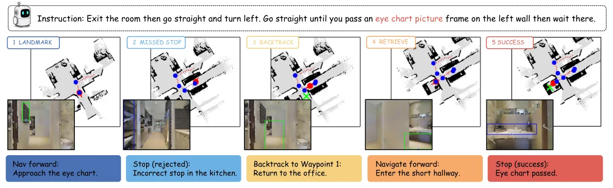
Figure 4: An instance of reflection-memory-driven backtracking. After a rejected stop in the kitchen the agent writes a note, backtracks to Waypoint 1 (office) to reorient, retrieves that note at the hallway intersection, takes the correct branch, and stops successfully.
The paper gives the full verbal trace: after a rejected stop in the kitchen the agent records "I will backtrack to Waypoint 1 (office) to reorient myself and find the hallway with the eye chart picture frame on the left wall." At the hallway intersection System 2 retrieves that note, selects the short hallway, passes the eye chart, and stops successfully. This is the most direct evidence for grounded failure memory, because the note simultaneously contains a spatial reference (Waypoint 1, office), a semantic landmark (the eye chart picture frame), and a relative orientation (left wall). All three must be carried by place states on the graph, otherwise the note could not be reused once recalled.
Limitations
The paper has no dedicated limitations section, but two author-stated boundaries appear in the discussion of results. First, the authors explicitly concede that the strongest supervised systems still achieve higher SR and SPL on both R2R and RxR, and they offer a mechanism: agentic exploration samples directions under uncertainty while learned policies take shortcuts. What HAM-VLN buys is zero training cost and cross-benchmark generality, not the absolute precision ceiling. Second, evaluation rests on 100-episode subsets, and the authors need to cite prior work (subset SR within 1.1 points of the full split) to defend comparability, which is itself a methodological concession.
The following are my own additions from a systems-design perspective. First, the cost is reduced but not eliminated. Each episode still consumes 244.9k API tokens of Gemini-3.1-Pro calls, roughly 13 decisions per episode, which is neither small for real-robot latency nor for the bill. The paper compares token counts only; it reports no wall-clock latency and no dollar cost per episode. Second, the dependence on depth and odometry is strong. Building the world graph requires $\Gamma(O_t,D_t,P_t)$, i.e. depth back-projection plus odometry pose. Both are clean in simulation. On hardware, depth noise, glass and reflective surfaces, and odometry drift would enter the graph's geometry and topology directly, and the paper contains no real-robot or noisy-perception experiment. Third, the hyperparameters were never searched. $(\alpha,\beta,\gamma)=(1.0,0.3,0.3)$, $\rho=0.85$, $K_s=3$, $K_p=5$, and $K=1$ are identical across all three benchmarks. "No retuning needed" is presented as a virtue, but it also means retrieval sensitivity is uncharacterized; for long RxR instructions, whether $K_p=5$ suffices to cover the number of places one instruction touches is left unanswered. Fourth, failure evidence is advisory with no invalidation mechanism. A note surfaces only when its place is retrieved and never affects scoring. When the environment itself changes (a door opens, an object is moved) or when the note was simply wrong, nothing decays or revokes it, and repeated visits to the same place will keep feeding the same faulty note back into context. Fifth, semantics stop at place and category granularity. Object nodes carry open-vocabulary descriptions and soft attributes, but the graph has no instance-level identity and no cross-room object permanence, so instructions such as "follow the person you just saw" or "go back to the table where I put the cup" are outside the current representation.
Summary and Outlook
HAM-VLN's contribution is not a new memory store. It is handing write authority over memory back to the model that makes the decision, and attaching that memory to a sparse, depth-grounded world graph. Three design decisions carry the results: writes share the decision call (so cost does not increase), history is retrieved conditioned on the current subgoal instead of stacked chronologically (so context does not grow), and failures persist as place-level evidence instead of being discarded (so retracing becomes information). Tables 3 and 4 together show that none of the three is decoration: removing the graph costs 9.3 SR points; replacing the graph with full raw history triples tokens while leaving SR 7.7 points lower; removing reflection memory costs 11.2 SPL points.
For people deploying navigation on real robots, the transferable parts are clear. Implement memory as a structured state updated at decision frequency, not as a text buffer summarized afterwards. Add topology expansion to retrieval, because in navigation semantic similarity and reachability frequently disagree. Model failures explicitly as recallable negative evidence, but keep them advisory so exploration is not pruned prematurely. Equally important is what the paper does not touch: real sensor noise, real-time budgets, and long-horizon graph maintenance (cluster drift, broken topology) all remain simulation assumptions here.
Following the paper's own logic, three directions come next: persisting the world graph across episodes so a robot can reuse known topology in repeated environments; giving failure evidence time and confidence dimensions so it can decay and be overridden by new evidence; and lifting place-level semantics to instance level so memory can support long-horizon instructions that require object identity.
SOURCE LINKS