SSTG-Nav: Metric-Grounded Spatial-Semantic Topological Graphs for Reusable Object Navigation

Paper Metadata

Title: SSTG-Nav: Metric-Grounded Spatial-Semantic Topological Graphs for Reusable Object Navigation

Authors: Daojie Peng (HKUST Guangzhou), Bingtao Wang (Shandong University), Jun Ma (HKUST, corresponding author)

Links: arXiv:2608.00527 (https://arxiv.org/abs/2608.00527 , v1, 1 Aug 2026, primary cs.RO); project page https://daojiepeng.github.io/SSTG-Nav

Code and data status: released. The benchmark repository https://github.com/DaojiePENG/sstg-nav-bench ships the full pipeline (mapping, RGB-D grounding, fusion, retrieval, recovery, evaluation) together with unit tests; evaluation uses the HM3D-Semantics v0.2 ObjectNav validation split (1,000 episodes, 36 scenes).

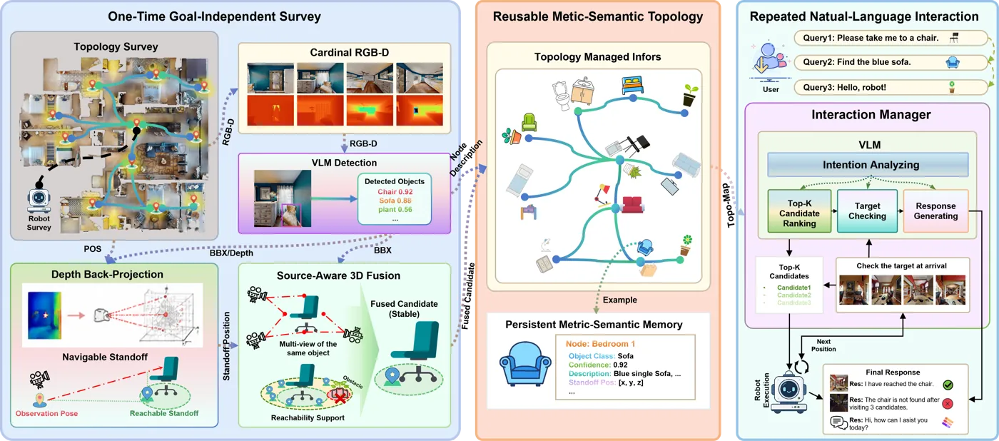
Figure 1: SSTG-Nav converts a one-time, goal-independent survey into a persistent metric-semantic topology that serves repeated natural-language navigation requests (paper Figure 1). Left: survey and RGB-D grounding; middle: topology-managed index and persistent metric-semantic memory; right: interaction manager driving retrieval, ranking, recovery, and arrival verification.

One-Sentence Summary

The paper reframes ObjectNav from "explore again for every request" to "survey once, reuse for a lifetime": a goal-independent farthest-point topology hosts view-local VLM detections, depth back-projection plus a 0.8 m standoff converts "recognized object" into "reachable stopping pose", and source-aware noisy-OR fusion with a residual-standoff second memory layer lifts one-shot success to 0.926 and Top-3 success to 0.975 on the full HM3D-v2 validation split.

Background and Motivation

ObjectNav asks an embodied agent to reach an instance of a requested category and declare STOP at a valid location. Mainstream benchmarks deliberately start the agent in an unexplored scene, and semantic exploration, vision-language frontier maps, commonsense constraints, online scene graphs, and topological memories have pushed success rates high in that regime. The operating reality of service robots is the opposite: the same home, office, or care facility is revisited hundreds of times, and repeating a full discovery for every request wastes prior perception and makes completion time unpredictable.

The paper therefore isolates a regime that prior work treats as a favorable assumption: reusable ObjectNav. The objective shifts from single-episode exploration efficiency to dependable completion over the robot's lifetime. A persistent map amortizes expensive perception, answers later language queries immediately, retains several hypotheses for ambiguous objects, and recovers from a rejected candidate without restarting search.

The scientific difficulty of this regime is making memory actionable. A camera may recognize an object through a doorway, across a railing, or from the wrong side of furniture, yet the camera pose itself is a poor navigation goal: it can be unreachable, on the wrong side of the object, or too far to declare success. The authors name this the observation-pose / STOP-pose mismatch and treat it as the gap between a reusable map and an executable goal.

A second difficulty is evidence independence. Neighboring nodes observe the same object repeatedly; counting duplicate boxes from one frame as separate confirmations inflates confidence, while collapsing a cluster to a single representative destroys the alternative stopping geometry needed when the primary hypothesis is rejected. The paper addresses both directions with source-aware fusion plus retained residual standoffs.

A third difficulty is the information boundary of evaluation. If map construction uses official goal viewpoints, successful STOP configurations are pre-baked into the map and success is systematically overstated. The paper therefore defines three protocols that separate target-view coverage, goal-independent geometry with oracle semantics, and goal-independent geometry with real VLM semantics, so every gain can be attributed to geometry, semantics, or representation design.

Preliminaries

Evaluation follows the Habitat 2023 Navigation Challenge ObjectNav protocol. For episode $e$ with requested category $c_e$, official shortest-path length $\ell_e$, and valid goal-viewpoint set $\mathcal{Y}_{c_e}$, a selected candidate $\hat{\mathbf{s}}_e$ succeeds when its navmesh geodesic distance to the nearest valid viewpoint is at most one meter:

$$S_e=\mathbf{1}\!\left[\min_{\mathbf{y}\in\mathcal{Y}_{c_e}}d_{\mathrm{geo}}(\hat{\mathbf{s}}_e,\mathbf{y})\leq 1\,\mathrm{m}\right]$$

Path efficiency is SPL, $\mathrm{SPL}_e=S_e\,\ell_e/\max(\ell_e,p_e)$ with executed path length $p_e$; DTG is the final geodesic distance to the nearest valid viewpoint. These metrics judge only whether the stop is correct and the route economical, so representation quality must be attributed through controlled ablations.

The information boundary of the three protocols is the key to reading every table. Target-view coverage captures four views at one high-IoU official navigable viewpoint per annotated instance; it measures semantic retrieval under controlled coverage and is not deployable. Independent oracle samples the map without goals and assigns oracle labels post hoc from the official goal sets, isolating geometric coverage. Independent real, the primary protocol, hides episode starts, categories, object annotations, and valid viewpoints throughout construction, capture, VLM inference, projection, fusion, and retrieval; they enter only after candidate selection to score success and DTG.

Method

5.1 Goal-Independent Spatial Topology

Per scene, a fixed-seed pool of 12,000 navigable points is drawn from the navmesh, then greedy farthest-point sampling starts at the pool point nearest the pool centroid and repeatedly adds the point farthest from the selected set until every pool point lies within 0.8 m of a selected node. The full validation split yields 6,642 nodes and 21,845 edges, with per-scene counts from 74 to 399: sampling stops on a coverage radius rather than a fixed node count, so compact apartments and large houses share one rule. Edges connect up to eight Euclidean neighbors and are kept only when a navmesh route exists, the Euclidean distance is at most 2.4 m, and the geodesic length is at most 3.84 m. No episode field is read during sampling, capture, inference, or fusion.

Every node stores four cardinal RGB-D views (yaw offsets 0/90/180/270 degrees) at 1.25 m camera height. Views are sent to the VLM separately rather than as a stitched panorama: panorama coordinates are ambiguous and stitching would destroy each view's camera model. Each detection is a tuple $d=(c,b,q,k)$ of category, normalized box, confidence, and view index.

5.2 From Detection to Navigable Candidate: Metric Grounding

Given box center $\tilde{\mathbf{u}}$ and the median of valid depths in a $7\times 7$ patch (accepted range 0.2-6.0 m), the surface point is back-projected with intrinsics $K$ and the world-from-camera transform $T_{wk}$:

$$\hat{\mathbf{o}}_{d}=T_{wk}\left(zK^{-1}[\tilde{\mathbf{u}}^{\top},1]^{\top}\right)$$

Expanded in pixel coordinates this is supplementary Eqs. (5)-(6): $x_c=2(u-0.5)\,z\tan(\phi_h/2)$, $y_c=-2(v-0.5)\,z\tan(\phi_v/2)$, $z_c=-z$, with vertical field of view $\phi_v=2\tan^{-1}\!\left(\frac{H}{W}\tan\frac{\phi_h}{2}\right)$. The standard camera is 640x360 with 90 degrees horizontal FoV (about 59 degrees vertical); the wide camera is 640x640 with 120 degrees in both axes. Depth is used purely as geometry here; semantic confidence remains the VLM output.

Observation poses are frequently unsuitable for stopping, so the surface point is shifted toward the source camera in the ground plane by $\rho=0.8$ m to obtain a standoff stopping pose:

$$\mathbf{s}^{*}_{d}=\hat{\mathbf{o}}_{d}+\rho\,\frac{\Pi(\mathbf{p}_{i}-\hat{\mathbf{o}}_{d})}{\|\Pi(\mathbf{p}_{i}-\hat{\mathbf{o}}_{d})\|_{2}}$$

where $\Pi$ drops the vertical coordinate. The candidate is snapped to navigable space and discarded when no navmesh path exists from the source node. Figure 2 shows an audited sofa observation: the view-local box indexes aligned depth, the median surface point is back-projected and shifted to a reachable 0.8 m standoff, and no ObjectNav goal information enters the construction. In the released code this chain lives in sstg_bench/rgbd_fusion.py: project() implements the Habitat camera convention (+X right, +Y up, -Z forward, sensor 1.25 m above the agent state), and candidate_from_detection() performs the standoff shift, snap_point snapping, and a shortest-path reachability test that returns None for unreachable candidates.

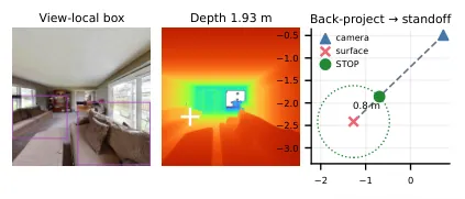
Figure 2: An audited sofa observation. A view-local VLM box indexes aligned depth; the median surface point is back-projected and shifted 0.8 m toward the source camera into a reachable standoff (paper Figure 2).

5.3 Reachability-Aware Soft Fusion and the Two-Layer Memory

Detections of one category form a cluster only when their object estimates lie within horizontal radius $r_o=1.2$ m and vertical tolerance $r_h=1.0$ m, and their STOP candidates are mutually reachable within geodesic threshold $r_g=3.0$ m. The third condition is essential: Euclidean proximity alone merges observations across walls or between disconnected floor levels. Duplicate boxes from one source node contribute only their maximum confidence, and the noisy-OR score is computed over independent observing nodes:

$$Q(C)=1-\prod_{i\in U(C)}\left(1-\max_{d\in C_{i}}q_{d}\right)$$

with $U(C)$ the set of independent source nodes. On the full-validation map a cluster is retained with at least two source nodes or a singleton confidence of at least 0.92; the minival representation controls retain every valid cluster so that category scarcity is not confounded with filtering. Fusion compresses 20,107 valid depth candidates into 1,329 representatives, a 93.4 percent reduction.

The paper stores two linked layers. $\mathcal{H}^{F}$ holds one $Q$-scored representative standoff per retained cluster for stable primary ranking; $\mathcal{H}^{R}$ keeps every reachable pre-fusion standoff with its view-local confidence for recovery. In sstg_bench/rgbd_fusion.py the source_confidence dictionary first takes the per-source maximum and only then multiplies, with a comment stating that independent observations raise confidence while duplicate boxes from the same frame must not inflate support; every retained cluster member is additionally persisted as a multi_standoff node so query-time Top-K can keep the fused semantic score while choosing distinct reachable stopping poses.

Before any of these numbers exist, the mapping stage must complete reliably, and the supplementary completion audit (Table 4) records that it does: all 6,642 node-level GPT-5.4 requests on the full split finish, yielding 21,579 raw detections, 20,107 valid depth candidates, and 1,329 fused candidates at a provider-reported 44,499,374 tokens. Both hosted backends share one parser version, bbox-norm-or-1000-v2, which accepts coordinates in [0,1] or [0,1000], clamps bounds, and rejects invalid boxes and categories, so model comparisons do not confound response scaling. The local Qwen2.5-VL-3B control consumes a 2x2 grounding panorama instead of four separate views; a subset of panoramas degenerates under deterministic decoding and is repaired by re-prompting the four original views independently, with the repair mode recorded in the immutable detection cache so that camera-node, raw, and fused variants all read identical detections.

5.4 Arrival Verification: Deciding STOP from Fresh RGB-D

The deployed loop never reads the goal set. After arriving at candidate $k$ the robot captures four fresh 120-degree RGB-D views: view zero faces the stored object estimate and the others rotate by 90 degrees. The VLM receives these views plus the boxed mapping-time reference and returns target visibility, a stopping-side judgment $g_k$, an arrival-view box, and confidence $q_k$; the central half of that box indexes aligned depth with median $z_k$. STOP is accepted exactly when

$$A_k=\mathbf{1}\!\left[\mathrm{visible}_k\wedge g_k=\mathrm{valid}\wedge q_k\geq 0.75\wedge 0.25\,\mathrm{m}\leq z_k\leq 2.5\,\mathrm{m}\right]$$

On rejection, planning continues from the current pose to the next spatially diverse candidate instead of restarting the episode. The 1,000 raw-list episodes reference 656 unique candidates and produce 2,624 fresh views; all 656 verifier requests complete, at a mean latency of 20.52 s per unique candidate.

5.5 Reusable Query and Execution Layer

A language normalizer maps query $q$ to category $c(q)$, and the fused primary candidate set is $\mathcal{C}(q)=\{i:c_i=c(q),\ \mathbf{s}_i\text{ reachable from }\mathbf{x}_0\}$. Ordering is the lexicographic permutation

$$\boldsymbol{\pi}_q=\operatorname{LexSort}_{i\in\mathcal{C}(q)}\left(-Q_i,\ d_{\mathcal{G}}(\mathbf{x}_0,\mathbf{s}_i)\right)$$

which makes semantic support the primary key and path length a deterministic tie-breaker. This prevents a nearby unsupported observation from outranking independently corroborated evidence while avoiding a learned query-time policy. Visit one takes $\pi_q(1)$; up to two later visits are drawn from the category-matched residual set $\mathcal{R}(q)\subset\mathcal{H}^{R}$ ordered by confidence and path distance while enforcing $\|\mathbf{s}_i-\mathbf{s}_{\pi_q(j)}\|_2\geq 2$ m separation from every prior visit; if $\mathcal{C}(q)$ is empty the best reachable residual becomes visit one.

Execution is a receding candidate sequence: leg $k$ is $P_k=\operatorname{ShortestPath}(\mathcal{G},\mathbf{x}_{k-1},\mathbf{s}_{\pi_q(k)})$ with $\mathbf{x}_k=\mathbf{s}_{\pi_q(k)}$, and the executed path is $P(q)=P_1\oplus\cdots\oplus P_\tau$ for $\tau=\min\{k:A_k=1\}$. Ordering costs $O(m_c\log m_c)$ and each graph search $O(|\mathcal{E}|+|\mathcal{V}|\log|\mathcal{V}|)$; if one survey serves $N$ requests the amortized non-motion cost is

$$\bar{C}_N=C_{\mathrm{map}}/N+C_{\mathrm{retrieve}}+C_{\mathrm{plan}}$$

so VLM inference and depth grounding are paid once while repeated requests perform retrieval, graph search, and fresh arrival verification only. In the code, sstg_bench/topk.py::diverse_candidates() greedily skips nodes closer than min_separation to an already selected candidate, hierarchical_candidates() implements the primary-then-residual layering, and the rank key (-score, distance) is exactly Eq. (7).

flowchart TB
  subgraph SURVEY["One-time goal-independent survey"]
    A[FPS topology 6642 nodes
21845 edges, cover radius 0.8 m] --> B[4 cardinal RGB-D views per node]
    B --> C[View-local VLM detection
category, box, confidence, view index]
    C --> D[7x7 patch median depth]
    D --> E[Back-project surface point Eq.2]
    E --> F[0.8 m standoff Eq.3
navmesh snap + reachability test]
  end
  subgraph FUSE["Source-aware fusion"]
    F --> G[Cluster by 1.2 m horizontal
1.0 m vertical, 3.0 m geodesic]
    G --> H[Noisy-OR over unique sources Eq.4]
    H --> I[H^F one representative per cluster]
    H --> J[H^R all residual standoffs]
  end
  subgraph QUERY["Repeated natural-language query loop"]
    K[Query normalized to category] --> L[LexSort by -Q then path length Eq.7]
    I --> L
    L --> M[Leg k: graph shortest path Eq.8]
    M --> N[Fresh 4-view RGB-D arrival check Eq.5]
    N -->|accept: q at least 0.75, depth 0.25-2.5 m| O[STOP and report completion]
    N -->|reject| P[Next residual at least 2 m apart]
    J --> P
    P --> M
  end

Figure 3 (schematic): SSTG-Nav data flow as specified by Algorithm 1 and Section 3.4 of the paper. The survey pays perception once, fusion produces the two-layer memory, and the query loop executes candidates receding-horizon style with a fresh RGB-D verdict at each arrival.

Experiments

The main study runs on the 1,000 HM3D-Semantics v0.2 validation episodes (36 scenes, six categories: chair, bed, plant, toilet, TV/monitor, sofa) with GPT-5.4 as the primary semantic backend and MiMo-v2.5 plus local Qwen2.5-VL-3B as model controls; representation and model ablations use the 30-episode, two-scene minival subset on a 339-node graph. Table 1 places the result across operating regimes: the strongest unknown-scene system, ConsistNav, reports 0.842/0.412, while a single fused SSTG-Nav destination reaches 0.926/0.586 and fusion-aware Top-3 reaches 0.975/0.601, margins of 0.133 SR and 0.122 SPL. The comparison crosses regimes by design: the reusable map amortizes perception over repeated requests, and the paper makes that difference explicit through the amortized cost formula rather than pretending a like-for-like race.

Method	Scene at start	Evaluation	Policy	SR	SPL
ConsistNav	unknown	HM3D-v2	TF	0.842	0.412
IntentNav	unknown	HM3D-v2	learned	0.822	0.385
TrajRAG	unknown	HM3D-v2	TF	0.781	0.402
FOM-Nav	unknown	HM3D-v2	learned	0.758	0.479
CARe+VLMaps	pre-explored	custom MP3D	TF	0.827 (dagger)	-
SSTG-Nav fused, single	pre-explored	HM3D-v2	TF	0.926	0.586
SSTG-Nav fusion-aware Top-3	pre-explored	HM3D-v2	TF	0.975	0.601

Table 1: Cross-regime context (excerpt of paper Table 2). The dagger marks CARe's self-reported custom MP3D success metric, which is not directly comparable.

The coverage-semantics decomposition (paper Table 3) localizes the gains. Target-view coverage with oracle semantics gives 0.990/0.802, so even privileged coverage is not perfect; with real Qwen semantics it collapses to 0.644/0.438, attributing a 0.346 gap purely to semantic retrieval. The goal-independent topology with oracle semantics reaches 0.994/0.992, proving that 0.8 m farthest-point sampling covers nearly every success region; with GPT-5.4 fusion the system lands at 0.926/0.586. Geometry is near its ceiling; the remaining bottleneck is semantic grounding and STOP placement, not map density.

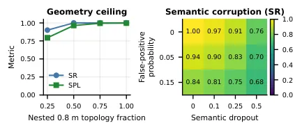
Figure 4: Geometry saturates before semantic reliability (paper Figure 3). Left: oracle SR/SPL on nested topology fractions 0.25/0.50/0.75/1.00 (about 85/170/255/339 nodes); right: mean SR over 20 seeds of the label-corruption grid, columns are dropout probability and color encodes false-positive probability.

Figure 4 sharpens that reading. On minival, half density (about 170 nodes) already saturates oracle SR at 1.000, whereas the corruption panel shows 25 percent label dropout cutting mean SR to 0.907, 50 percent dropout to 0.763, and 15 percent false positives to 0.840; combining 50 percent node retention, 25 percent dropout, and 15 percent false positives drops mean SR to 0.602. Geometry saturates early while modest semantic corruption remains damaging: the most informative contrast in the paper.

Map protocol	Semantics	Nodes	SR	SPL	DTG
Target-view	Oracle	1,168	0.990	0.802	0.073
Target-view	Qwen	1,168	0.644	0.438	2.016
Independent	Oracle	6,642	0.994	0.992	0.622
Independent	GPT-5.4 fused	6,642	0.926	0.586	0.747

Table 2: Coverage-semantics decomposition (paper Table 3). Target-view capture poses derive from official goal viewpoints; independent maps never see them.

The cumulative same-response ablation (paper Table 4) prices each component. The camera-node baseline sits at 0.835/0.560; adding metric grounding raises it to 0.920/0.603 with 93 gains versus 8 losses under an exact McNemar test ($p=1.74\times10^{-19}$), the largest and most significant single-step gain in the paper, achieved without changing any semantic prediction. Adding source-aware fusion moves SR to 0.926 but SPL down to 0.586 (28 gains, 22 losses, $p=0.480$), indicating that at full scale fusion buys candidate compression and ranking stability rather than net success. Adding residual recovery lifts Top-3 to 0.975/0.601. The sequential recovery ablation in Table 3 separates recovery strategies: fused-only Top-3 saturates at 0.964, whereas one primary representative plus two 2 m-separated residuals reaches 0.975 with eleven paired gains and no losses (nine sofa, two bed), showing that recovery works by preserving stopping geometry that fusion suppresses, not by visiting more clusters.

Candidate policy	K	SR	Delta SR	SPL	Successes
Single fused target (no recovery)	1	0.926	-	0.586	926
Fusion-aware primary only	1	0.928	+0.002	0.588	928
Fused-only Top-3 control	3	0.964	+0.038	0.596	964
Primary + one diverse residual	2	0.965	+0.039	0.598	965
Primary + two diverse residuals	3	0.975	+0.049	0.601	975

Table 3: Sequential recovery on full validation (paper Table 6). Delta SR is measured against the strict single fused target.

The same-response triplets (paper Table 5) test whether fusion is merely a prompting artifact: across all six backend-by-FoV combinations fusion raises raw SR, from 0.920 to 0.926 at full scale, 0.867 to 0.967 and 0.933 to 1.000 for the GPT controls, 0.333 to 0.500 for Qwen, and 0.833 to 0.900 plus 0.567 to 0.633 for MiMo. Wider field of view is not a free gain: GPT-5.4 at 120 degrees reaches 1.000 SR because fusion replaces an unsupported sofa singleton with a 22-source cluster and exposes a low toilet, while MiMo falls from 0.900 to 0.633 when widened, showing that visibility, projection geometry, and VLM localization must be calibrated together. Figure 5 ties the aggregate numbers to individual cases: wide capture grounds a successful toilet standoff, source-aware fusion replaces an unsupported sofa singleton with a 22-source hypothesis, fresh RGB-D rejects a wrong rank-1 plant and accepts a spatially distinct rank-2, and the physical sequence shows the Yahboom X3 pipeline from RGB-D alignment and persistent topology to language retrieval of a toy at Node 22 and Nav2 arrival.

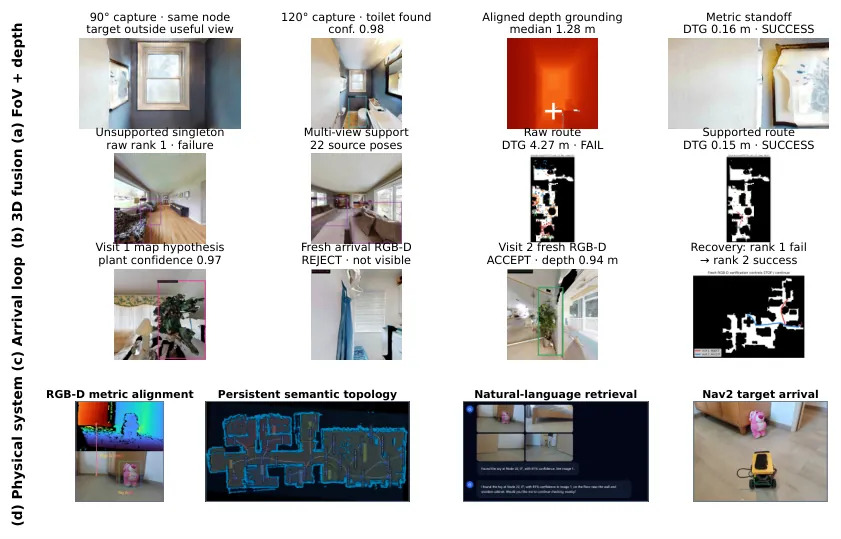
Figure 5: Mechanism and deployment audit (paper Figure 4). (a) Wide capture and depth ground a successful toilet standoff; (b) source-aware fusion replaces an unsupported sofa singleton with a 22-source hypothesis; (c) fresh RGB-D rejects a wrong rank-1 plant and accepts rank 2; (d) physical sequence: RGB-D alignment, persistent semantic topology, language retrieval at Node 22, Nav2 arrival.

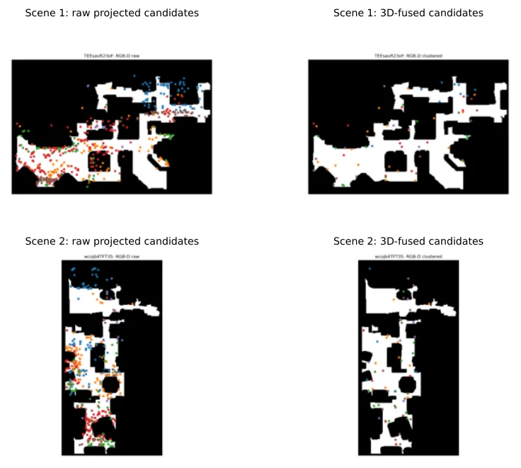
Figure 6: Actual semantic maps for both minival scenes (supplementary Figure 1). Left columns show every valid depth-projected candidate; right columns show candidates surviving 3D and reachability clustering. Fusion removes repeated projections while retaining category coverage across floors.

The per-category audit (supplementary Table 6) shows where the representation helps and where it does not. Under goal-independent GPT-5.4 mapping, metric grounding lifts chair from 0.841 to 0.974 SR and plant from 0.862 to 0.941 after fusion, while toilet is already strong at the camera-node stage (0.934) because its distinctive geometry survives even ungrounded retrieval. The two categories that expose the remaining ranking-efficiency tradeoff are bed and sofa: bed peaks at the raw RGB-D stage (0.988) and loses 0.012 SR under fusion, and sofa falls from 0.914 to 0.893, because collapsing a cluster to one representative can discard the stopping side that a particular episode needs. These per-category movements are exactly why the paper keeps the residual layer: the fused index stabilizes ranking, and the residuals restore the geometry that ranking suppressed.

The arrival verifier deserves separate attention because it is the only component that closes the loop without oracle information. Over the 656 unique candidates of the raw-list protocol, the strict dual-geometry rule (visibility, valid stopping side, confidence at least 0.75, and measured depth in [0.25, 2.5] m) ends 912 of 1,000 episodes successfully, with accepted ranks 1/2/3 accounting for 888/55/3 of the accepts; against the post-hoc official success test it reaches precision 0.964 and recall 0.915 at 1.110 attempts per episode on average. Two ablations sharpen the design choice: dropping the stopping-side flag and keeping only category plus RGB-D range raises recall slightly (0.924) but lowers precision (0.956), and running the same verifier over the collapsed fused candidate list loses both (0.947/0.891), which is the empirical reason the final hierarchy lets fusion control the primary hypothesis while residual metric standoffs remain available for Top-3 recovery. In other words, the verifier and the two-layer memory were co-designed against each other's failure modes rather than stacked independently.

The physical realization runs on a Yahboom X3 mobile robot with ROS 2 Humble and Nav2 executing metric goals, a Gemini 336L supplying aligned RGB-D, an RPLIDAR S2 supplying laser scans, and slam_toolbox maintaining occupancy mapping and localization; a persistent manager retains the graph and interaction state across legs. The illustrated query retrieves a toy at Node 22 with 0.81 confidence before dispatching the selected target to Nav2. The paper states plainly that all quantitative SR/SPL numbers come from simulation and the physical sequence documents qualitative system integration only.

Limitations

The authors' own scope statement covers one HM3D-v2 split, one hosted primary VLM, six categories, and static scenes; continuous navmesh paths abstract away control noise and map change; relational dialogue such as "the vase next to the sofa" lies beyond the category-query benchmark and is not quantitatively evaluated; hosted endpoint weights and future serving behavior are outside the authors' control; and the reported intervals quantify episode sampling uncertainty only, not cross-dataset, model-serving, or real-world variation.

Three independent judgments follow from the tables. First, the full-scale net success gain of fusion is not significant (28 gains versus 22 losses, $p=0.480$) and SPL shows a small but resolvable decrease (delta SPL -0.017, 95% CI [-0.032, -0.002]); the abstract headlines "fusion reaches 0.926", yet Tables 4-7 support the reading that fusion's value is compression and ranking stability while recovery supplies the net success. Second, arrival verification costs a mean 20.52 s per unique candidate (median 19.45 s, P95 32.31 s) on top of 44,499,374 hosted tokens for the full survey, and the paper reports neither end-to-end wall-clock time nor a cost accounting, leaving the deployment economics open. Third, every quantitative claim rests on simulated navmesh shortest paths; motion blur, localization drift, and collision recovery are absent, and their effect on verifier precision and recall is unmeasured even though the verifier is the only safety valve in the closed loop.

Conclusion and Outlook

The contribution of SSTG-Nav is not a single trick but the conversion of reuse from a favorable assumption into a rigorously evaluated operating regime: three information-boundary protocols isolate geometry, grounding, fusion, and recovery; metric grounding delivers the largest and most significant single-step gain; the two-layer memory with 2 m-separated residuals pushes Top-3 success to 0.975; and a ROS 2/Nav2 realization shows the interfaces survive contact with a real robot. For robots that live in the same environment for months, paying perception once and reducing later requests to retrieval and graph search is closer to deployment reality than any per-episode exploration strategy.

The open problems are equally concrete. Semantic grounding remains the bottleneck (0.994 oracle geometry versus 0.926 real semantics), and open-vocabulary or relational queries demand new representations and benchmarks. Map aging, object motion, and verifier recalibration under dynamic environments are unaddressed. And the MiMo counterexample warns that wide-FoV and fusion gains do not transfer automatically when the hosted VLM is replaced by an on-device model; each backend needs its own calibration. The authors plan to extend the persistent-map and arrival interfaces to dynamic environments and broader real-camera evaluation.

Golden Quote

Recognizing an object is not knowing where to stop: the true product of reusable navigation is not a map, but a set of corroborated, reachable, and verifiable stopping poses.