RelateAnything: Real-Time Open-Vocabulary Relation Prediction From Any Inputs

Paper: RelateAnything: Real-Time Open-Vocabulary Relation Prediction From Any Inputs (arXiv:2609.12552v1)
Author: Maëlic Neau (independent researcher, no institutional affiliation)
Code and data: released. GitHub repository Maelic/RelateAnything; HuggingFace hosts the model maelic/relateanything and the corpus maelic/RA-4M; the project page ships an in-browser demo
Content type: open-vocabulary scene graph generation / visual relationship detection, with a direct link to indoor robot perception through IndoorVG

In One Sentence

RelateAnything moves the relation vocabulary out of the model parameters and into a string argument passed at inference: a 53.2M-parameter relation head takes an image plus regions from any source, scores them against a bank of 19,103 predicate embeddings in 20 milliseconds per frame, and reaches 2.3x to 3.5x the mean recall of the strongest comparable open-vocabulary system across datasets.

Background and Motivation

Open-vocabulary detection and promptable segmentation have already finished de-taxonomizing themselves: a detector accepts an arbitrary class list at inference, a segmentation model returns regions without needing class names at all. The taxonomy is no longer part of the model, it is an input to the model. Relation prediction has stayed where it was. Scene graph models still train and evaluate on the 50 predicates of Visual Genome or the 56 of PSG, and the relation head is conditioned on object class labels, which binds the model permanently to one detector and one annotation style.

The paper traces that stagnation to three obstacles and is explicit that none of them is a modeling problem. First, supervision: there is no relation corpus that is both free-text and verified, and machine-generated corpora never validate their own annotator. Second, architecture: a relation head conditioned on object labels cannot accept vocabulary it did not see during training, so changing the vocabulary means retraining. Third, metrics: standard recall rewards agreement with the training corpus, a pixel-free frequency lookup can win the leaderboard metric, and therefore a larger vocabulary reads as a regression under the old metric.

The three obstacles interlock. The frequency lookup is strong precisely because it recites the annotation prior of the training corpus, and a model that takes object labels as input inherits that prior for free, together with the part of it that does not transfer. Table 1 of the paper is the sharpest evidence: on per-edge top-1 accuracy the pixel-free frequency baseline beats the trained model by roughly 15 points on all three benchmarks, while on per-predicate macro-averaging the same predictions let the model win back 29% to 86%. The lookup returns the majority predicate for each class pair; micro metrics reward exactly that behaviour and macro metrics punish it. The conclusion is narrow but sharp: a metric that a pixel-free lookup can win is not measuring relation understanding, and it happens to be the metric used to rank the leaderboard.

For robot systems this is not an academic complaint. The indoor scene graph benchmark IndoorVG, contact and support relations in manipulation, and the ordinary need to swap a detector for a tracker or a segmenter without retraining the relation model all require the relation head to be decoupled from object labels. The paper answers with three artifacts: a verified free-text relation corpus, RA-4M; a label-agnostic relation model, RelateAnything; and a cross-dataset six-axis evaluation protocol, OV-SGG-Bench.

That also fixes the stance of the paper. It does not chase scores under the old protocol; it first argues that the old protocol measures the wrong thing, and then reports every result under the new one. Not one in-domain number appears as a headline result anywhere in the text. Every cell comes from images and annotations excluded during training, and each is accompanied by the triplet overlap between the training corpus and the benchmark so that readers can judge for themselves how much of a number is prior matching.

Primer: What Scene Graph Evaluation Actually Measures

The standard protocol for scene graph generation is this: given an image and regions, either ground-truth boxes or detections, predict a predicate for each ordered object pair and report recall as R@K and mR@K. mR computes recall per predicate and then averages, so it is sensitive to the long tail, while R@K is dominated by head predicates. The paper notes that recall metrics reward three priors: shared triplet mass, meaning the training corpus and the benchmark annotated the same ternary relations; the object class prior, since a class pair very nearly determines the predicate; and annotation propensity, since some pairings are simply more likely to be annotated.

The second variable that is usually ignored is the scoring convention. Whether the matcher allows synonym tolerance, whether it forces one-to-one assignment, the detector confidence threshold and the box cap: each of these moves results more than the differences between methods do. The paper measures that the detector operating point alone explains 4.3 points of the gap across all published OvR-SGG methods, and that pair recall is quadratic in object recall, so detector recall is a ceiling for any relation model.

OV-SGG-Bench therefore defines six opportunity-corrected axes: A1 cross-dataset transfer, A2 precision on human-adjudicated negatives, A3 full-vocabulary openness, A4 real-detector mode, A5 graph quality without ground truth, and A6 adversarial spatial negatives. The composite score is the harmonic mean of the opportunity-corrected axis values, and only a system that runs on all axes gets one.

Method

Input Contract: Pixels, Regions, Strings

The model takes three separable things: one frame, a set of regions from any detector or segmenter with their class labels discarded, and the predicate vocabulary supplied as strings at inference time. The output is a set of scored triplets (i, j, p). Two constraints follow. Object labels are never a network input; they appear only inside two loss terms, the relevance loss of the sampler and the object-text grounding term. And there is no learned transform on the text side, because a projection fitted to the training vocabulary is undefined for a string handed in later. Changing the vocabulary is therefore a matter of replacing a matrix, not of retraining.

Visual Path: Encode Once, Pool Everywhere

A DINOv3 backbone, ViT-S/16+ and larger, encodes the image at 448x448 and reads patch features at depths -6, -3 and -1, applying layer norm per tap before fusing them with learned weights. Object features are not crops but coordinate-aware soft pooling: the query is built from the Fourier position encoding of box b_i and attends over all patch tokens,

$$v_{i}=\mathrm{Attn}(q(b_{i}),F,F)$$

so an object's representation can carry the context it interacts with. The backbone is fully fine-tuned at a learning rate eight times lower than the head.

Pair Representation: The Contact Region Is a First-Class Feature

The representation of an ordered pair concatenates five feature paths and projects them to 512 dimensions:

$$x_{ij}=\big[\,v_{i};\;v_{j};\;v_{\cup(i,j)};\;v_{\cap(i,j)};\;\mathrm{MLP}(g_{ij})\,\big]\,W_{\mathrm{proj}},\qquad x_{ij}\in\mathbb{R}^{512}$$

Here v_union pools the union box, v_cap pools the contact region, which is the intersection when the boxes overlap and the gap between them otherwise, and g_ij is a 19-dimensional scale-invariant geometric feature made of 15 box features plus 4 mask-only slots. A small Transformer refinement follows: self-attention over the sampled pairs, cross-attention to scene tokens and to the pair's own box-corner tokens, then a joint self-attention over pairs and scene. The last stage is additive: each pair predicts sampled offsets around four anchors and reads the feature map through a zero-initialized gate. That stage is what makes parked on depend on the road surface and hanging from depend on the attachment point above the subject.

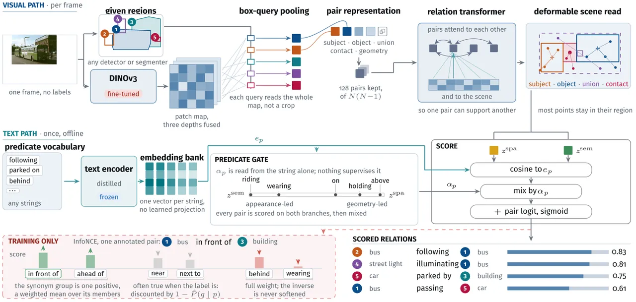
Figure 1: RelateAnything overview. The top band is the visual path, where the region source is not part of the model and its labels are discarded; the middle band is the text path and the predicate-conditioned gate; the bottom band is the training-only loss structure. Source: paper Fig. 2 / project-page architecture diagram.

Dual Branches and the Predicate-Conditioned Gate

Spatial and semantic relations rely on different evidence, so the head scores every pair twice and mixes the two cosine channels per predicate:

$$\ell_{\mathrm{pred}}(i,j,p)=\tau\big[\alpha_{p}\cos(z^{\mathrm{spa}}_{ij},e_{p})+(1-\alpha_{p})\cos(z^{\mathrm{sem}}_{ij},e_{p})\big]+\beta$$

where e_p is the text embedding of the predicate and alpha_p = g(e_p) depends only on that embedding, so it is defined for strings never seen in training. The gate receives no direct supervision, yet the learned weights are strongly bimodal: projection and proximity relations route to the geometric branch, behind at 1.000, below at 0.9998, above at 0.970; actions route to the appearance branch, carrying at 0.0004, parked on at 0.0008, riding at 0.012; contact predicates sit in between, holding at 0.82, on at 0.64, wearing at 0.22. The median is 0.002 and only 12% of predicates exceed 0.5. Because both branches score before mixing, a single forward pass yields the layout graph and the content graph at once.

Sampling: From N(N-1) Pairs to 128

The two-stage sampler first keeps 400 of the N(N-1) ordered pairs by geometric plausibility, then keeps 128 by a learned relevance score, retaining 99.79% of annotated positives; exhaustive scoring costs 1.02x and buys nothing measurable. The learned stage is trained to predict which pairs carry annotations, so what it learns is annotation propensity. Its logit enters the final score additively, which means it can be removed at evaluation time and its contribution measured on its own.

Positive-Unlabeled Supervision Under Ten Thousand Predicates

The model trains against 19,103 free-text predicates: the 10,102 of RA-4M itself plus 9,001 drawn from the vocabularies of three other relation corpora, using their vocabularies only and none of their relations. The main objective is in-batch InfoNCE, where positives are the synonym group of the annotated predicate, weighted by estimated synonym probability and averaged, and negatives are the other predicates in the batch. With 50 predicates, treating unlabeled as negative is roughly correct; with ten thousand it is systematically wrong. If (man, horse) is annotated as riding, then sitting on and mounted on are true but unwritten, and penalizing them teaches the model to suppress correct answers.

The paper's fix is a positive-unlabeled discount. For every ordered predicate pair it estimates the probability that q also holds when p is annotated, fitting on co-occurrence counts over 706k multiply-annotated box pairs plus text-space cosine and frequency, with an Elkan-Noto correction to separate unlabeled from false. The denominator logit for a negative q becomes

$$\ell_{\mathrm{pred}}(i,j,q)+\log\big(1-\hat{P}(q\mid p)\big)$$

Predicate pairs that are almost surely co-true contribute almost nothing to the denominator, and pairs with several annotations are discounted by combining them independently. Two exemptions are mandatory: an annotated predicate is never down-weighted, and directional antonyms such as above and below always keep full weight, because telling up from down is exactly the supervision that must not be softened. On the positive side, synonym weights come from an isotonic fit on text cosine over 1,177 lexical synonym pairs, and a directional swap hinge

$$\mathcal{L}_{\mathrm{swap}}=\max\big(0,\;m-c(i,j,p)+c(j,i,p)\big),\qquad m=0.05$$

weighted by the directionality probability of each predicate puts subject-object order into the loss. No semantic constant anywhere in the objective is hand-set.

Text Space: Antonyms Must Be Separated

The head regresses visual features onto text directions, so the geometry of the text space bounds what the model can express. Contrastive text encoders fail exactly on the dimension relations depend on most: antonyms appear in nearly identical contexts, so their embeddings end up nearly identical. The teacher encoder, dino.txt at 2048 dimensions, places above and below at cosine 0.95, in front of and behind at 0.94, to the left of and to the right of at 0.99, indistinguishable from the 0.96 average of its synonym pairs. Removing the mean direction does not rescue it.

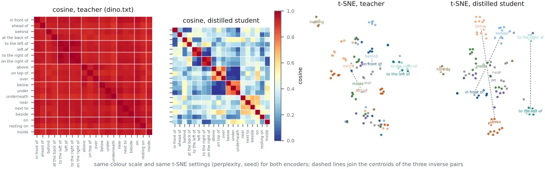
Figure 2: Teacher and distilled student text spaces. The two left columns show pairwise cosine over 20 spatial predicates, the two right columns show t-SNE over 10 synonym families. The teacher mixes antonym pairs into one cluster; the student keeps synonym blocks, pushes antonym blocks to near zero and splits them into two clusters. Source: paper Fig. 3.

The solution is to distil a 512-dimensional student encoder over the full CLIP BPE vocabulary, so that no predicate string can ever fall out of vocabulary. Among the five objectives, the antonym repulsion hinge on known antonym pairs is the one a frozen teacher cannot provide, and the neighborhood preservation term stops the student from buying separation cheaply: without it the student reaches the same synonym/antonym AUC at an effective dimensionality of 24 instead of 44. After distillation that AUC rises from 0.85 to 0.99, the mean antonym cosine falls from 0.92 to 0.09 while synonyms stay at 0.71, and hubness falls from 8.1 to 1.3. The student is used offline only; at inference the model carries the embedding bank.

RA-4M: Verifiable Machine Annotation

The corpus is generated by open-weight vision-language models of the Gemma family over images carrying numbered marks: one coloured dot at the centre of each box holds the box index, which makes grounding an input to the annotator rather than something inferred backwards from its output. Every candidate relation then passes a deterministic geometric gate that rejects 11.3% of raw candidates. The gate fires only where box geometry logically constrains the predicate, so a rejection is a true negative up to box annotation error, while predicates that geometry cannot constrain pass through unchanged and are counted as residual risk. Behind the gate, 0% of containment relations and 0.1% of contact relations have disjoint boxes, and the corpus has no duplicate triplets and no self-loops. Direction repair is the only gate that does not reject: left/right and above/below swap subject and object according to the boxes, and every verified directional relation is then restated from the other end with probability one half, leaving the corpus directionally balanced.

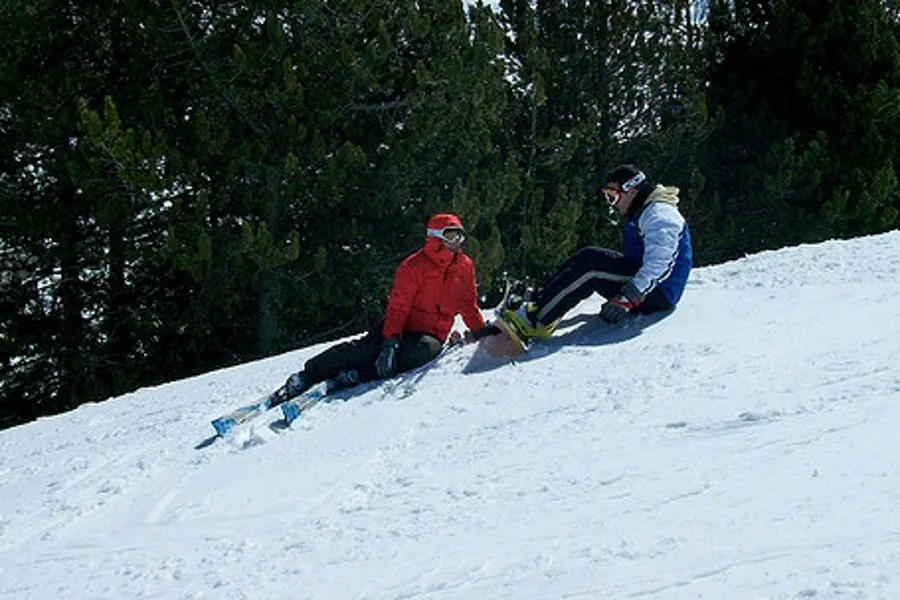
Figure 3: A RA-4M corpus image: one frame, several regions, and one free-text relation verified by the geometric gate. Source: paper Fig. 1, left.

The final corpus holds 474,413 images, 4,282,531 relations and 10,102 distinct free-text predicates, at 9.03 relations per image and 104 GPU-hours of generation cost. Against the source annotations on the same images and boxes, RA-4M is 1.7x denser, 9.03 versus 5.29, has 107x the vocabulary, carries 1.4 nats more predicate entropy, and reproduces 73 of the 94 source predicate classes as exact strings. The distribution is still long-tailed, with the top ten predicates at 57%, but the head is now made of directionally balanced spatial predicates such as behind, in front of, wearing, to the right of and to the left of; mean object degree rises from 1.88 to 3.20 and the share of single-connected-component images from 70.9% to 82.6%.

flowchart TD
  A["Input frame 448x448 no object labels"] --> B["DINOv3 ViT-S/16+ patch features taps -6 -3 -1"]
  R["Any region source detector or segmenter class labels discarded"] --> P["Coordinate-aware soft pooling v_i = Attn q(b_i) F F"]
  B --> P
  P --> C["Ordered pair representation subject object union contact region geometry MLP projected to 512 dims"]
  C --> S["Two-stage sampling N times N minus 1 to 400 then to 128"]
  S --> T["Pair transformer self-attention across pairs cross-attention to scene"]
  T --> D["Deformable scene readout four anchors zero-initialized gate"]
  D --> Z["Dual branches z_spa and z_sem"]
  V["Predicate strings at inference frozen student embeddings bank of 19103"] --> G["Predicate-conditioned gate alpha_p = g(e_p)"]
  G --> M["Per-predicate cosine mix plus pair logit plus temperature and bias"]
  Z --> M
  M --> O["Scored relation graph 20 ms per frame compiled"]
  subgraph TRAIN["Training only"]
    L["InfoNCE synonym-group positives positive-unlabeled discounted negatives"]
    E["Student text encoder antonym repulsion plus neighborhood preservation"]
  end
  E --> V
  Z --> L

Figure 4: The real method flow drawn from Section 3 of the paper: how the visual path, the text path, the predicate-conditioned gate and the training-only objectives connect.

Results

A1: Cross-Dataset Transfer

All four benchmarks are cross-dataset: unseen images, unseen object distributions and unseen annotation styles, with the single exception of the annotated HICO-DET row. RelateAnything receives no object labels; the baseline OvSGTR receives ground-truth labels. The result is a lead on every metric of every source: head recall is 1.04x to 1.40x the baseline, mean recall 2.3x to 3.5x, and rare-bucket recall 5x to 21x, where the ratio is undefined on VG150 because the baseline rare recall is exactly 0.0. The triplet overlap column explains where the gap comes from. VG150 is OvSGTR's own benchmark, with 90.9% of its training triplet mass overlapping the benchmark versus 12.8% for this model, and the baseline's flagship number on that row is carried by 21 high-frequency predicates, exactly the part recoverable without any visual input.

Benchmark	Triplet overlap	OvSGTR R@50	OvSGTR mR@50	OvSGTR F1@50	RelateAnything R@50	RelateAnything mR@50	RelateAnything F1@50
VG150	13%	39.9	10.4	16.5	53.3	28.2	36.9
PSG	11%	28.7	8.8	13.5	40.1	30.6	34.7
IndoorVG	7%	48.1	12.8	20.2	52.7	29.5	37.8
HICO-DET (zero-shot tower)	-	34.0	4.5	7.9	35.3	12.7	18.7

Table 1: Axis 1, cross-dataset transfer (paper Table 4). Same test sets, ground-truth boxes, graph constraints and evaluator; the baseline gets ground-truth object labels, this model does not.

Six Axes and the Composite

Not one of the six axes is in-domain. A2 measures precision on human-adjudicated negatives: mean fAP 72.6 versus 52.1 and rare-predicate fAP 70.7 versus 44.6, which shows the recall advantage was not bought by asserting wildly. A3 takes the answer set back: the model answers from all 19,103 strings and is matched with synonym tolerance, giving R@50 of 56.0 on VG150, higher than the 53.3 obtained when the 50 benchmark strings are handed over, and the median rank of the ground-truth string among the 19,103 candidates is 1 on VG150 and IndoorVG and 10 on PSG. A4 runs under a shared YOLO-World detector: wR@50 of 20.0 versus 4.0, while the pair-recall ceiling is only 69.6. A6 uses adversarially collected SpatialSense negatives: macro AUC 69.0 versus 59.1, with a box-only baseline at 68.8, meaning that on the spatial axis the model has only just passed "geometry alone".

Axis	Metric	Best baseline	RelateAnything
A1 transfer VG150	F1@50 (mR@50)	19.6 (15.2) ROBIN-3B	36.9 (28.2)
A1 transfer PSG	F1@50 (mR@50)	27.9 (22.9) ROBIN-3B	34.7 (30.6)
A1 transfer IndoorVG	F1@50 (mR@50)	22.7 (21.5) ROBIN-3B	37.8 (29.5)
A2 precision	mean fAP (rare fAP)	52.1 (44.6) OvSGTR	72.6 (70.7)
A3 open vocabulary	mR@50, VG/PSG/Indoor	20.9 / 25.1 / 25.4 ROBIN-3B	34.5 / 28.3 / 34.6
A4 detector mode	wR@50 (mR@50)	4.0 (6.2) OvSGTR	20.0 (20.5)
A5 graph quality	true bits per graph (share of annotated)	13.4 (0.48) OvSGTR	18.6 (0.67)
A6 spatial	macro AUC (pooled AUC)	59.1 (61.7) OvSGTR	69.0 (67.5)
OVS composite	harmonic mean of opportunity-corrected axes	11.8 (OvSGTR only)	40.1

Table 2: OV-SGG-Bench six axes and composite (paper Table 3). The baseline column is the envelope of two systems; the composite is computed for OvSGTR alone.

Free-Text Systems on the Open-Vocabulary Axis

A3 also hosts a family of baselines that fit nowhere else: ROBIN-3B, built on a 3B vision-language backbone, plus general multimodal models such as Qwen3-VL, InternVL3.5 and GLM-4.6V. With ground-truth regions, one shared set of generations and different matchers, the matcher itself turns out to be worth more than the difference between methods: mapping free text onto the benchmark vocabulary adds 11.7 R@50 for ROBIN and 23.2 for this model. Under synonym-tolerant matching this model reaches macro recall 31.3 against ROBIN's 25.1, while micro recall is still led by ROBIN. The two metrics point in opposite directions, exactly the shape the prior analysis predicted. Pair coverage is the more stable signal: 99.7% for this model, 45.6% to 77.4% for ROBIN, and 23.1% to 35.5% for the general models. A pair that is never named cannot carry the right predicate, and scale mostly buys coverage.

Graph Quality: Information, Not Edge Count

A5 faces the question of how to compare two graphs when there is no ground truth. The paper lets a vision-language judge decide only whether each relation is true, then prices each accepted relation by its surprisal under a reference distribution:

$$I=\sum_{r:\,\mathrm{judge}(r)=\mathrm{true}}-\log_{2}p_{\mathrm{ref}}\!\left(\mathrm{pred}(r)\right)$$

The two factors cover each other's blind spots. Surprisal alone rewards rare predicates emitted at random, which the judge then rejects; truth alone rewards on, worth 2.31 bits, over riding, worth 7.04 bits; and neither can be inflated by repetition. At equal depth, the top ten pairs per system, this model reaches 18.6 true bits per image against 13.4 for the baseline; at each system's own deployment depth the numbers are 28.7 versus 14.1. The judge acceptance rate is slightly higher for the baseline, 4.33 versus 4.07 out of 9.8 relations per image, but the information per accepted relation is 3.09 versus 4.57 bits: the baseline's graph is safer and more redundant.

Decoupling Objects From Relations: The Probes Say No

Section 7 asks whether relation supervision leaves a relation representation in the shared backbone. The answer is no. Fine-tuning raises class selectivity from 0.242 to 0.281 while relation selectivity barely moves, from 0.133 to 0.138, and the probability that a relation partner is more similar than an unrelated object of the same class drops from 0.469 to 0.385 against a chance level of 0.500. The contact region does change: its advantage over distant subject patches rises from 0.356 to 0.438 and the feature moves from covering the whole person to covering the hand and the object. But what it encodes is object identity. Cross-image 1-NN retrieval reaches 0.761 for the object class against a chance of 0.068, and only 0.269 for the verb against a majority-class chance of 0.424, below chance.

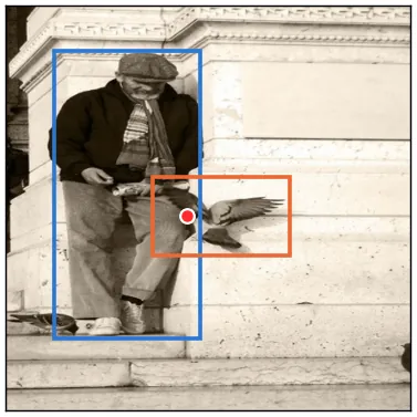
Figure 5: Contact-region similarity maps. Before fine-tuning a hand query highlights the whole person; after fine-tuning it highlights the hand and the bird. Querying from the bird side returns the same region, which shows the region encodes which object is being manipulated rather than what is being done. Source: paper Fig. 7.

The attribution side is equally clean. An input-channel ablation ladder shows that removing pixels costs 44% to 68% of micro accuracy, removing box geometry costs 6% to 24%, and removing the object-to-text channel costs 0.1%. In the exact variance decomposition of the semantic logit, pair context accounts for 87% to 93%, subject features for 0.1% and object features for 0.0%. In the label-dependence experiment, 88% to 90% of the baseline's outputs are reproduced by a majority-predicate table over its own label pairs and shuffling the labels leaves its output statistics unchanged; this model cannot see labels at all, and its residual 69% lookup overlap is a class prior recovered from pixels, people wear clothes and cups sit on tables.

One Model, Two Region Sources

The direct payoff of decoupling is that the region source becomes replaceable. With one checkpoint, one calibrated operating point at p greater than or equal to 0.45, which happens to emit PSG's own density of 6.0 edges per image, and one 19,103-predicate bank, open-vocabulary boxes from YOLOE-11 and class-free masks from FastSAM both produce valid relation graphs: 8 relations per image on the detection row, 18 on the segmentation row. Object names are used for display only and never enter the model.

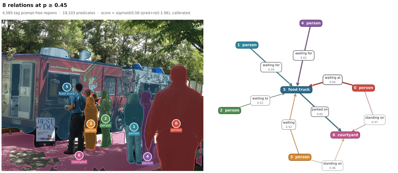
Figure 6: Output of the same checkpoint over YOLOE-11 detection regions, 8 relations per image at p greater than or equal to 0.45. Source: paper Fig. 6, top.

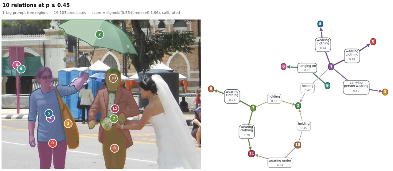
Figure 7: Output of the same checkpoint over class-free FastSAM masks, 18 relations per image. The region source and the taxonomy are both replaced and the model is not retrained. Source: paper Fig. 6, bottom.

Cost: Real-Time Is Not a Side Effect

Under a unified protocol at batch 1 in eager PyTorch, OvSGTR with a Swin-T backbone, 177M parameters, 98 boxes per image, 800/1333 resolution and fp32 runs at 194.0 ms on an A40, that is 5.1 FPS. This system, 231M parameters of which 53.2M is the relation model, 20 boxes per image, 448 px and bf16, runs at 25.0 ms, that is 40 FPS, or 7.8x faster end to end. At batch 1 the cost is dominated by kernel dispatch rather than arithmetic: all three towers land between 19 and 20 ms within a 2.5x range of FLOPs. Compilation buys 1.5x to 1.8x and pushes the whole chain, detector and decoding included, to 20 ms per frame. Scoring 19,103 strings costs under 1 ms at batch 1 and 11% to 22% of throughput when batching. The text encoder sits outside the inference graph and the detector is not part of the model, so the same graph runs on a CPU: the fp16 build reaches 7 FPS on 8 threads with 0.955 top-1 agreement against fp32.

System	Parameters	Boxes/img	A40 ms	A100 ms	H100 ms	FPS (A40)
OvSGTR Swin-T	177M	98	194.0	179.9	128.1	5.1
OvSGTR Swin-B	237M	98	228.5	195.1	134.3	4.3
RelateAnything + YOLO-World	231M	20	25.0	35.0	25.6	40.0

Table 3: End-to-end cost under the unified protocol (paper Table 11). What is compared is a deployment configuration rather than an architecture: the box budget is the largest of the three differences.

In-Domain Versus Cross-Dataset: Transfer Overstated Five Times

Section 8 reads corpus size under both regimes at once. In-domain validation recall rises with the number of training samples and the half-corpus arm saturates after the third pass, while the transfer curve tells a different story: in-domain measurement overstates the transfer gain by about five times and may even favour changes that reduce transfer. This is the most uncomfortable and most useful number in the paper, because it says that many of the changes that "work" under the old protocol are ineffective or actively harmful under deployment conditions.

Limitations

The corpus has no human precision audit (stated by the author). Every precision claim about RA-4M is structural: the gate rejects 11.3%, rejections are true negatives up to box error, and predicates that geometry cannot constrain are named and counted rather than inspected. The author explicitly acknowledges the missing measurement, a batch of generated relations read and scored by a human, and calls it the estimate readers should expect and should add first before relying on 4.3M machine annotations. The residual error classes are named too: about 22% of looking at / watching annotations have disjoint boxes and cannot be verified; prior-driven labels on large boxes; and contact predicates between overlapping but unrelated boxes, where person wearing tent passes the contact gate.

Predicate concepts are not truly held out (stated by the author). All unlabeled results are cross-dataset, but the predicate strings are not: every benchmark predicate appears in the training vocabulary. Held-out variants are evaluated only on the split that defines them, and the general variant that holds concepts out across all four benchmarks at once was not run, even though the architecture allows it since the predicate matrix is never learned. Some conclusions rest on a single seed, and differences inside the 1.3% noise floor are flagged by the author.

The A5 judge does not always side with this model (stated by the author). Per-relation precision is a real weakness: at any depth the baseline over-asserts less, and a deployment that cannot tolerate false edges should prefer the shorter graph. When whole graphs are shown the judge prefers the baseline's graph, when single relations are shown the judge accepts the baseline slightly more often, and a second judge reproduces the finding. Methodologically, the judge cannot perceive duplication, so information must be measured against a reference distribution rather than elicited by asking.

Detector recall is a hard ceiling (stated by the author). The largest loss between benchmark numbers and the deployed system comes from object detector recall: pair recall is quadratic in object recall and no relation model can get past it, while a larger relation model only buys precision on rankings the deployment never emits.

Conclusion and Outlook

The contribution of RelateAnything reads as three moves outward: the vocabulary moves out of the parameters, into an embedding bank plus a predicate-conditioned gate; object labels move out of the input, into coordinate-aware soft pooling plus a label-agnostic head; and the metric moves out of a single corpus, into a six-axis cross-dataset protocol with triplet overlap disclosed. Together they make the relation head, for the first time, a component whose detector can be swapped, whose vocabulary can be swapped, and that runs in real time. For robot systems that need to replace the perception stack with a tracker or a segmenter, that has direct engineering value.

The negative result from the probes matters just as much. Under this recipe, relation supervision does not produce a relation representation in the shared backbone, and the relation logit is almost entirely determined by pair context. That is a counterexample to the default practice of sharing a backbone between detection and relations, and it points to the next step: patch-level relation objectives, rather than another larger relation head.

The unfinished list is equally clear: a human precision audit, predicate hold-out across benchmarks, multi-seed reproduction, and false-edge control at deployment depth. The cheapest recommendation in the paper is worth adopting for all scene graph work: report the shared triplet mass between the training corpus and the benchmark next to every recall number.

Golden Lines

"Detection and segmentation have escaped the taxonomy; relation prediction has not. We argue the obstacles are supervision, architecture and metrics, and we remove one of each."

"A metric that a pixel-free lookup can win is not measuring relation understanding - and it is the metric that ranks the leaderboard."