OPEN SOURCE DEEP DIVE
mjbatch: Batched MuJoCo Simulation on a CPU Thread Pool
A small Python + C++ library from Kevin Zakka that steps thousands of MuJoCo simulations in parallel on the CPU through a single Batch object: C++ thread pool execution with the GIL released, bind() giving live array views across the whole batch, and expand() for per-simulation model parameters. Memory scales with thread count rather than simulation count, so 4096 simulations stay under 256MB; on a 24-thread machine with a Unitree G1 scene it measured 10.3x over a serial mj_step loop, reaching 676,019 sim-substeps per second with ten substeps batched per call. The repo ships six self-contained solver examples spanning iLQR, predictive-sampling MPC, PPO reinforcement learning, CEM hardware co-design and damped Gauss-Newton system identification, including a Go1 joystick controller that learns to walk in under a minute on a five-year-old M1 laptop.
One Model, Thousands of Simulations, No Accelerator
Most of the interesting work in robot simulation is not one trajectory, it is a population of them. A trajectory optimizer needs a bundle of rollouts to finite-difference a gradient. A sampling MPC needs a thousand candidate action sequences per control step. A reinforcement learning run needs a thousand environments so the policy update is not dominated by variance. A system identification fit needs the same recorded motion replayed against seventy candidate inertia vectors. Every one of those workloads is embarrassingly parallel across simulations and completely serial inside each one, which is exactly the shape that a multicore CPU handles well and a single-threaded Python loop handles terribly.
mjbatch is a small Python and C++ library from Kevin Zakka that targets precisely that gap: it steps thousands of MuJoCo simulations in parallel on the CPU, exposed as a single Python object, with the GIL released for the duration of the physics call. It released as version 0.1.0 under Apache-2.0 on 10 September 2026, pins mujoco==3.11.0, and ships wheels for CPython 3.10 through 3.14 including the free-threading build. The whole library is two headers and one binding file, plus a thin Python wrapper for named accessors.
benchmarks/scaling.py stepping 256 Unitree G1 simulations on a 12-core / 24-thread machine. Throughput climbs from 8,530 sim-substeps per second on one thread to 88,111 on twenty-four, and batching ten substeps per call lifts the same 24-thread configuration to 676,019.The Whole API Is One Object
The model is copied at construction, so you edit the MjModel before you hand it over and never mutate it afterwards. Calls are serialized: one step at a time, no concurrent reentry.
import mujoco, numpy as np
from mjbatch import Batch

model = mujoco.MjModel.from_xml_path("scene.xml")
batch = Batch(model, num_sims=4096)          # threads default to every logical CPU
qpos, ctrl = batch.bind("qpos"), batch.bind("ctrl")
batch.expand("geom_friction")[:, :, 0] = np.random.uniform(0.4, 1.2, (4096, 1))
for _ in range(1000):
    ctrl[:] = policy(qpos)                   # your controller, all 4096 at once
    batch.step()                             # qpos updates in place
num_threads=0 means every logical CPU, clamped to num_sims. That default is deliberate and the source carries the reasoning as a comment: MuJoCo's linear algebra is small and dense, so it stalls on latency rather than saturating a core, and running two threads per physical core measured 1.3 to 1.5 times the throughput of one on a Threadripper 7960X. The other constructor flag, forward=True, ends every step with mj_forward so derived fields are current with the state instead of one substep behind, at the cost of one forward pass per simulation per call.
| Method | Signature | Behaviour |
|---|---|---|
bind | bind(name, dtype=None) -> NDArray | A live (N, ...) view over an mjData field in MjData's own layout. bind("state") instead returns the raw (N, nstate) integration-state rows. |
expand | expand(name, dtype=None) -> NDArray | Per-simulation mjModel or mjOption values, seeded from the model and applied before every physics call. |
step | step(ids=None, nstep=1, history=None) | nstep mj_step calls per simulation on one worker. ids selects a subset as sorted unique ints or a boolean mask. |
forward / reset | forward(ids=None), reset(ids=None, keyframe=-1) | reset runs mj_resetData (or mj_resetDataKeyframe), applies pending writes, then mj_forward, so derived fields are valid immediately. |
set_const | set_const(ids=None) | Runs mj_setConst per simulation and expands every field it changed, making derived constants per-simulation too. |
On top of the C++ binding, the Python layer adds named accessors that mirror MjData's own: sensor("name"), joint("name"), actuator("name"), body("name") and site("name") each return live views sliced out of the bound fields. joint knows that a free joint occupies seven qpos columns and six qvel columns while a ball joint takes four and three, so batch.joint("floating_base").qpos is the right shape without you counting offsets.
Memory Follows Threads, Not Simulations
This is the design decision that makes 4096 simulations fit on a laptop, and it is worth stating precisely because it is not the obvious one. Each simulation stores only its mjSTATE_INTEGRATION vector plus warning counters. The mjData is per worker thread, not per simulation. Before each call, a worker loads the states of its assigned simulations into its own mjData, steps them, and writes the states back out.
The consequence is that memory cost is a function of thread count, which is a small fixed number, rather than simulation count, which you choose. The test suite pins this with a subprocess that measures ru_maxrss growth: allocating one mjData per simulation for 4096 sims grows resident memory by 712 MB on the test model, whereas 4096 state vectors are a few megabytes, and the assertion is that the batch stays under 256 MB. Models with sleep enabled are rejected at construction, because sleep bookkeeping lives outside mjtState and would silently desynchronize.
The same asymmetry explains the batched-substep result in the benchmark. Ten substeps per call amortizes the state load and store over ten physics steps instead of one, which is why the 24-thread column jumps from 88,111 to 676,019 sim-substeps per second. If your solver can tolerate not touching Python between substeps, nstep is the cheapest speedup available. examples/hello.py pushes this to its limit: 4096 pendulums released from 4096 different angles, stepped 1000 times in a single batch.step(nstep=1000) call, with the GIL released for the whole thing.
Live Arrays and the Copy Discipline
bind returns a real numpy array over a batch buffer, not a snapshot. Writing to it is how you set state and controls; reading it after a step is how you observe. The library keeps a mirror of what it last wrote for input fields, so the copy-in before a physics call is element-by-element and only touches what changed since the last write. Every bound field is copied out after the call, and a derived field bound between calls is filled for a simulation by its next call. Writing a row of bind("state") sets that simulation's state at its next call, with any pending field writes applied on top, and the field views stay stale until then. reset discards both, exactly as it discards a field write.
The dtype rules are mechanical: mjtNum fields are float64 (or float32 against a float32 libmujoco), float is float32, int is int32, mjtByte is uint8, mjtBool is bool, and you may ask for float32 explicitly on any mjtNum field. Against a float32 build that path is a plain memcpy.
expand is what turns a batch of identical simulations into a batch of different ones. It covers mjModel arrays such as geom_friction, body_mass and dof_armature, and it covers mjOption as well, scalars as (N,) and vectors as (N, size). So gravity, timestep, integrator and the solver settings are all per simulation, which is what makes domain randomization and per-environment physics parameters a one-line operation. Two caveats are documented in the binding itself. Raising iterations or ls_iterations, or switching cone to elliptic, can make a simulation need more arena than the template sized the worker's mjData for, and that surfaces as the usual trapped MuJoCo error naming it. And enableflags cannot turn sleep on, for the same reason the constructor rejects a sleeping model. Derived constants follow expanded inputs only after you call set_const, mirroring mj_setConst on a single model; mjModel scalars that mj_setConst writes, such as flags and stat, are kept per simulation as well.
What the Numbers Say
The benchmark harness, benchmarks/scaling.py, is honest about its baseline: the comparison point is one mjData stepped in a plain Python loop, 20 warmup substeps then 200 timed ones, and speedups are reported against that. It accepts a scene XML, a MuJoCo Menagerie model name, or an XML whose meshes Menagerie holds via --assets. The figures below are from the release run on a Unitree G1 scene with 256 simulations on a machine reporting 12 cores.
| Configuration | 1 substep per call | Speedup | 10 substeps per call |
|---|---|---|---|
Serial mj_step loop (one mjData) | 8,523 | baseline | not applicable |
threads=1 | 8,530 | 1.0x | 85,429 |
threads=8 | 58,217 | 6.8x | 487,360 |
threads=24 | 88,111 | 10.3x | 676,019 |
Two readings matter here. First, at threads=1 the batched path matches the serial loop to within a tenth of a percent, so the abstraction is not costing you anything when there is nothing to parallelize. Second, scaling from 8 to 24 threads buys 1.5x, not 3x, which is the expected shape for hyperthreaded small-matrix work: the first eight threads claim physical cores, the next sixteen share them. The 7.7x headroom between one thread and twenty-four is the prize, and the roughly 7.7x further headroom from batching substeps is on top of it.
The thread pool is where the engineering actually lives. It is a persistent pool with a blocking parallel-for and sticky slices: item i belongs to the slice of worker i * T / n, which keeps a given simulation on the same core across calls and therefore keeps its mjData warm in cache. A worker that finishes its own slice claims remaining items from the others through an atomic counter, so nobody waits on the slowest slice. Only one Run may be active at a time and the worker function must not throw, which is why MuJoCo errors are trapped rather than propagated as C++ exceptions.
Error handling deserves a sentence of its own because it changes how you write solvers. A MuJoCo error on any worker raises a RuntimeError naming the first failing simulation; the other simulations still ran to completion, and the failing one keeps the state it had before the call with its writes still pending. The trap is a MuJoCo log handler installed at import time, and installing another handler afterwards disables it.
Six Solvers, All Self-Contained
The examples are the argument that this primitive is enough on its own. Each is a single file with a complete solver, not a wrapper around a framework, and they span four families of method.
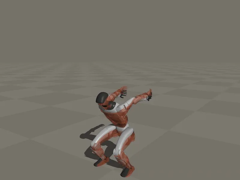
examples/g1_flip.py: a Unitree G1 tracking a mocap backflip with receding-horizon iLQR. The ghost is the reference clip, the solid robot is the tracked result. Fifty knots are planned per window, ten are committed, and twenty iLQR iterations run per window at 50 Hz control, two physics substeps per knot.The G1 backflip is the most demanding of the set. It tracks 200 frames of a retargeted mocap clip across twelve bodies, with per-square-metre and per-radian cost weights on position and orientation error, a Huber-like softening above a threshold so a large position error grows linearly rather than quadratically, and a root weight vector that is deliberately loose in x and y but 1000 times tighter in z. The clip's ankles roll after frame 200, so tracking stops there.
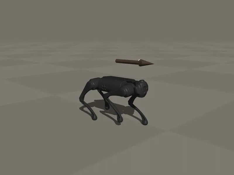
examples/go1_joystick.py: PPO on 1024 parallel Go1 environments. The README's claim is that the controller learns to walk in under a minute on a five-year-old M1 laptop. It ships a pretrained go1_policy.pt so you can play the result without training.The Go1 trainer is a complete PPO implementation in one file: 1024 environments, 24-step horizon, 600 iterations, 500-step episodes, a 4 ms timestep with decimation 5 for 50 Hz control, PD gains of 35 and 0.5 with the real rotor inertia of 0.000111842 kg m squared added as armature, and a 50-dimensional observation against 12 actions. Domain randomization redraws ground friction between 0.4 and 1.0 every five seconds, and the reward mixes velocity tracking, turn tracking, a 2 Hz trot gait term with the diagonal phase pairs, pose, orientation, bounce, wobble, joint limits and action rate. It puts the network on CUDA or MPS when available but keeps the actor on CPU under MPS, because for a net this small the transfer costs more than the compute.
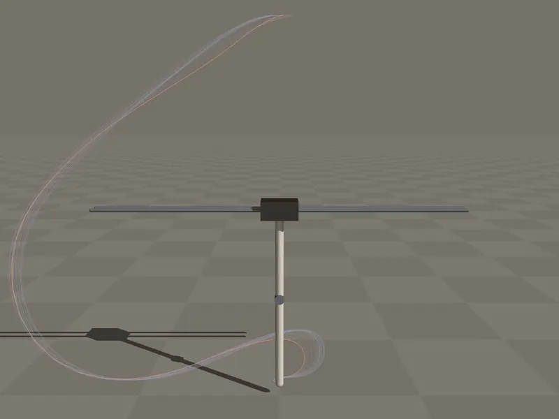
examples/cartpole_swingup.py: iLQR swinging up a cart carrying two poles. One hundred knots at four substeps each, six-dimensional state, one control, finite-difference gradients with a nine-step backtracking line search, and up to 300 iterations with a relative cost drop tolerance of 1e-4. The terminal knot is weighted 100 times the running cost.The two cartpole files show the same task solved two ways. cartpole_swingup.py runs iLQR with analytic gradients and Hessians of the cost along the trajectory, regularizing the negative diagonal that appears while a pole hangs below the pivot. cartpole_mpc.py runs predictive sampling after the method in arXiv 2212.00541: 1024 noisy rollouts over a 25-knot horizon, pick the best, commit the first four substeps, repeat for 150 headless control steps. Because a receding horizon never reaches a final knot, every knot carries the running cost. That second file is the clearest demonstration of why the library exists: 1024 rollouts per control step is a batch dimension, not a loop.
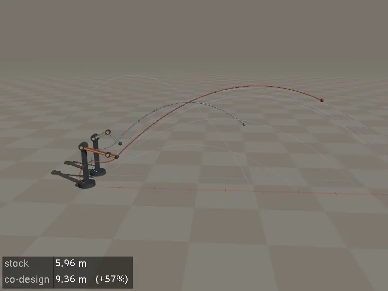
examples/arm_throw.py: cross-entropy method jointly optimizing a throwing arm's link proportions, gear ratios and torque knots. The search space is two link lengths, two gear ratios, a release deadline and eight control knots, sampled over a population of 512 for 30 generations with a 0.1 elite fraction. Each candidate is its own simulation, and expand is what gives each one different link lengths and gears.The throwing arm is hardware co-design rather than control. It fixes a 1 m reach and a 0.045 m ball radius, sets the integrator to implicit-fast with a 2 ms timestep and 40 solver iterations, restricts collisions to ball against floor, and then searches over morphology and control together. The motor model is real: 6 and 3 N m stall torques, 24 rad/s free speed, 0.0006 kg m squared rotor inertia, a 0.65 s deadline with four knots per motor. Without per-simulation model parameters this is a recompile per candidate; with expand it is a column write.
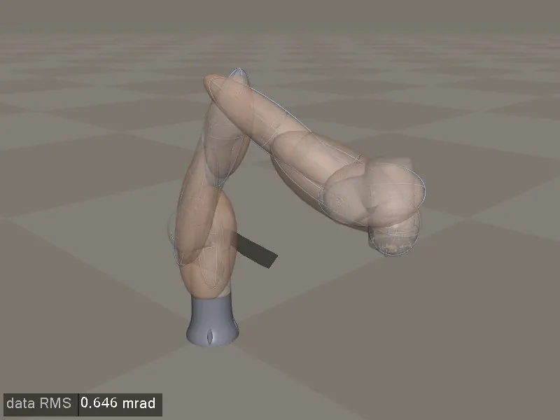
examples/rizon_inertia.py: damped Gauss-Newton fitting the inertial parameters of a Flexiv Rizon to synthetic motion data. Seventy unknowns, seven links by ten coordinates each, over body_mass, body_ipos, body_inertia and body_iquat, with a 0.35 standard-deviation prior in dimensionless CAD coordinates and 2e-4 radians of simulated encoder noise. Twenty-five iterations, five-step line search, tolerance 1e-5.The system identification example is the one that leans hardest on the batch-as-Jacobian idea. It records 1000 commands at 100 Hz, five physics substeps each, from a Rizon driven through a multisine excitation with per-joint amplitudes between 0.08 and 0.3 radians and frequencies between 0.37 and 1.07 Hz under realistic PD gains. Then it fits seventy parameters against that recording using finite differences with a 1e-6 step, which means each Jacobian column is another simulation. A 50-sample window per step keeps the batch small and the iterations frequent.
Packaging, Portability and the Honest Limits
The build is scikit-build-core with nanobind, and the packaging decisions are documented in comments rather than left implicit. Wheels are built for cp310 through cp314 plus cp314t, the free-threading build, which is a meaningful signal: a library whose entire job is releasing the GIL during physics calls is one of the few that gets strictly more useful in a no-GIL interpreter. Windows and musllinux are skipped, and the reason is specific: the mujoco wheel ships mujoco.dll with no import library, and the extension finds libmujoco by rpath, for which Windows has no equivalent. On Linux, auditwheel repair excludes libmujoco.so.3.11.0; on macOS, delocate-wheel excludes the matching dylib. Pinning mujoco==3.11.0 exactly is what makes that exclusion safe.
The test suite is twenty-nine tests in one file, covering the semantics this article has been describing: change-tracking copy-in, the staleness of derived fields, bind("state") sharing memory with the returned array, reset discarding pending writes, subset selection by ids and by boolean mask, and the memory-does-not-scale-with-simulations property. Development tooling is pytest, ruff and pyright with a two-space indent and a 100-column line length.
The limits are worth naming. Calls are serialized, so there is no way to have two batches stepping concurrently from one object. The model is copied at construction, so a change to your MjModel afterwards does not propagate; you edit, then construct, and use expand for anything that should vary per simulation. Models with sleep enabled are rejected outright. Raising solver iterations or switching to the elliptic cone can outgrow the arena the template sized for the worker's mjData, and that arrives as a trapped MuJoCo error rather than a silent slowdown. There is no GPU path: this is a CPU library by design, and the comparison to make is against MJX rather than against it. What you get in exchange is that your whole toolchain stays numpy, your debugger stays a debugger, and a laptop with no accelerator can train a quadruped walking policy in under a minute.
Running It
# the throughput benchmark on a Menagerie model
uv run python benchmarks/scaling.py unitree_g1 --num-sims 256 --threads 1,8,24

# 4096 pendulums, 1000 steps, one call
uv run examples/hello.py

# the examples that open a viewer need a display; --headless does not
uv sync --group examples
uv run examples/go1_joystick.py
uv run examples/g1_flip.py --play        # replays a saved solve
The examples write their solves to disk, so g1_flip.py --play loads g1_flip_plan.npz instead of re-running the optimizer. That separation matters for the expensive ones: you solve once, then iterate on the visualization.
SOURCE LINKS