OPEN SOURCE DEEP DIVE
Genesis World: The Unified Multi-Physics Simulation Platform for Physical AI
Genesis AI's open simulation platform for physical AI: one Pythonic API over a multi-physics engine (rigid, FEM, MPM, PBD, SPH, Stable Fluid, IPC), the Nyx path tracer, and Quadrants, a cross-platform Python-to-GPU compiler. It is built to be the evaluation engine for robot foundation models rather than a data factory: 30,000 parallel environments at 43M FPS, and under a zero-shot real-to-sim protocol, sim-vs-real evaluation agreement of Pearson 0.8996 with mean maximum rank violation 0.0166. Apache 2.0, 29.9k stars.
A Simulation Platform Built for Evaluation, Not Just Data
Genesis World is a simulation platform for physical AI: a unified multi-physics engine, a photorealistic renderer (Nyx), and a cross-platform Python-to-GPU compiler (Quadrants), all exposed behind one Pythonic API. The repository holds roughly 262 Python modules under genesis/ (about 5.9 MB of source), 122 runnable examples, and 89 test files, and ships on PyPI as genesis-world under Apache 2.0, requiring Python 3.10 to 3.13. At the time of writing the project carries 29.9k stars and 2,853 forks, with version 1.4.0 released on 6 September 2026.
Its history explains a lot of the design. The project started as an academic effort in December 2024 under the name Genesis, framed as "a generative and universal physics engine for robotics and beyond". The GitHub repository itself was created in October 2023. Over the past year the initial version was rebuilt into a more systematic framework, and development is now officially supported by the company Genesis AI. The rename to Genesis World came with that transition, and the May 2026 blog post The Role of Simulation in Scalable Robotics, Genesis World 1.0, and the Path Forward states the position clearly: simulation is treated as the evaluation and iteration engine for robotics foundation models, not merely as a data generator.
Four Layers, One Scene, One State
The architecture document and the README both describe the platform as four layers. Above them sits whatever you build (robotics environments, ML pipelines, data generation, agentic simulation); below sits whatever compute backend you happen to have.
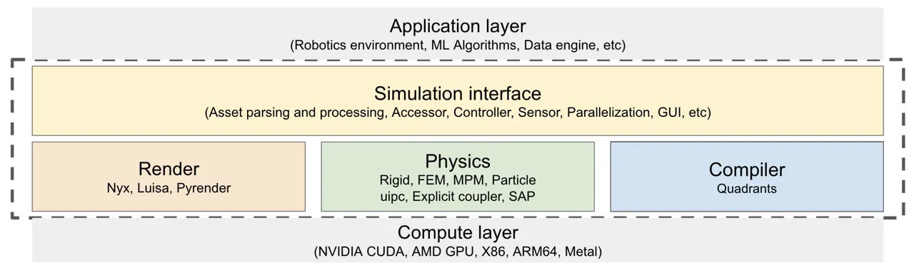
- Simulation Interface — the user-facing API: asset parsing (URDF, URDF xacro, MJCF, USD, OBJ, STL, GLB/GLTF), entity accessors, controllers, sensors, parallel and heterogeneous environments, and a built-in GUI.
- Physics — one engine integrating Rigid, FEM, MPM, particle (PBD / SPH), and Stable Fluid solvers plus
libuipc, with three interchangeable couplers resolving contact between them. Everything shares a single scene and a single state. - Render — three rendering paths that plug in as camera sensors: Nyx (in-house path tracer built for robotics), Luisa (a DSL ray tracer), and Pyrender (rasterizer).
- Compiler — Quadrants lowers Python kernel code to CUDA, AMD ROCm, Apple Metal, Vulkan, x86, and ARM64, and carries the autodiff, GPU-graph, and fast-cache machinery.
flowchart TB
    subgraph Above["What you build"]
        APP["Robotics environments · ML pipelines · data generation · agentic simulation"]
    end
    subgraph GW["Genesis World"]
        SI["Simulation Interface
URDF/MJCF/USD parsing · entities · controllers
sensors · parallel & heterogeneous envs · GUI"]
        PH["Physics
Rigid · FEM · MPM · PBD · SPH · Stable Fluid
one scene, one state"]
        RD["Render
Nyx path tracer · Luisa ray tracer · Pyrender rasterizer"]
        CO["Compiler: Quadrants
Python kernels → CUDA · ROCm · Metal · Vulkan · x86 · ARM64
autodiff · kernel graphs · fastcache"]
        SI --> PH --> RD --> CO
    end
    subgraph Below["Compute backend"]
        HW["Datacenter GPU · workstation GPU · laptop CPU"]
    end
    APP --> SI
    CO --> HW
Two convictions from the philosophy section shape everything below it. The engine is open source and written in Python, so there is no opaque binary between you and the physics: you can read it, debug it, and extend it. And the solvers are not bolted together at the edges — rigid, FEM, MPM, and particle solvers share one scene and one state, with the coupler resolving interaction exactly where their entities touch. The project also states that gradients flow through the physics by design, with reverse-mode autodiff in the compiler and hand-derived gradients for the hardest kernels.
One Solver per Material Family, Three Ways to Couple Them
Which solver runs is decided by the material you assign to an entity, not by a mode switch. MPM carries mass on particles while resolving forces on a background grid, which lets one solver span elastic solids, plastics, sand, and snow. FEM discretizes into a tetrahedral mesh and solves elasticity on it, and is what you pick when mesh-level accuracy matters: stiff elastic bodies, volumetric muscles, contact-rich soft-body manipulation. PBD represents an entity as particles linked by constraints and solves for positions directly, which makes it fast and stable for cloth and ropes. SPH is purely Lagrangian and aimed at free-surface liquids governed by real fluid parameters (rest density, viscosity, surface tension). Stable Fluid works on a fixed Eulerian grid, advecting a velocity field and scalar densities and then making the velocity divergence-free with Jacobi pressure projection, and gas enters through velocity jets rather than through an entity you add.
| Solver | Representation | Materials | Use it when you need |
|---|---|---|---|
| Rigid | Articulated links and geoms | gs.materials.Rigid | Robots and rigid objects from URDF / MJCF / USD |
| MPM | Hybrid particles + background grid | Elastic, Liquid, ElastoPlastic, Sand, Snow, Muscle | The widest range of continuum materials in one solver |
| FEM | Tetrahedral mesh | Elastic, Cloth, Muscle | Accurate elasticity, volumetric muscles |
| PBD | Particles + constraints | Cloth, Elastic, Liquid, Particle | Fast cloth, ropes, topology-preserving deformables |
| SPH | Lagrangian particles | Liquid | Free-surface liquids driven by physical parameters |
| SF | Fixed 3D grid (Eulerian) | velocity jets + density fields | Smoke and other gaseous phenomena |
Mixing them is the interesting part. The simulator instantiates exactly one coupler per scene, chosen by the options object you pass: SAPCoupler, LegacyCoupler, or IPCCoupler, with anything else raising at construction. The coupler exchanges state once per substep, which is why it is built only after the substep rate is known, and it runs as three hooks around the physics — preprocess(f), couple(f), and couple_grad(f) in the backward pass. Switching couplers is a one-line change with no change to assets, sensors, or the policy interface.
The fast general-purpose coupler handles the common pairings (cloth on rigid, rigid with MPM attachment, cutting, water wheels). The SAP coupler is a Drake-style Semi-Analytic Primal formulation with hydroelastic contact: the source computes a pressure field from unsigned contact distance scaled by a configurable hydroelastic_stiffness, and it maintains separate FEM and rigid hydroelastic field initializations with marching-tetrahedra edge tables for surface extraction. The IPC coupler wraps libuipc for intersection-free contact on delicate deformables, and it is where the most substantial new physics sits.
To couple IPC tightly to articulated robots, the team extended libuipc with an External Articulation Constraint that embeds joint-space dynamics directly into IPC's optimization, so joint-space forces and contact forces resolve simultaneously instead of being staggered between separate solvers. For an articulated system with $m$ joints, the rigid solver predicts joint displacements $\tilde{\delta\boldsymbol{\theta}}$ and computes the joint-space effective mass matrix $\mathbf{M}^t$, which is injected into IPC as an external articulation kinetic energy:
$$ K = \frac{1}{2}\left( \delta\boldsymbol{\theta}(\mathbf{q}, \mathbf{q}^t) - \tilde{\delta\boldsymbol{\theta}} \right)^T \mathbf{M}^t \left(\delta\boldsymbol{\theta}(\mathbf{q}, \mathbf{q}^t) - \tilde{\delta\boldsymbol{\theta}} \right) $$
where $\delta\boldsymbol{\theta}$ maps IPC affine-body states $\mathbf{q}$ to joint-space displacements. IPC minimizes this jointly with contact barriers, friction, and joint constraints. Without contacts the solver recovers the articulated prediction exactly; with contacts it deviates just enough to resolve them, weighted by effective mass so heavier links resist correction more. The source carries that intent literally: the uipc constitution imports include ExternalArticulationConstraint, AffineBodyRevoluteJoint, and AffineBodyPrismaticJoint, and the module defines a joint strength ratio of 100.0 with a default stiffness of 1e4.
On the contact-handling side itself, the team developed barrier-free elastodynamics to accelerate IPC-style simulation in contact-heavy scenes. Standard IPC enforces non-penetration with a logarithmic barrier, which makes the Hessian ill-conditioned for tight contact and slows active-set exploration because of the filtered line search. The replacement is a custom augmented Lagrangian: every contact pair returned by continuous collision detection enters the active set immediately, and constraint satisfaction is driven by adaptive Lagrange multiplier updates rather than escalating penalty stiffness. For each contact pair $i$ with linearized penetration depth $c_i(\mathbf{x})$, a slack variable $s_i$ converts the inequality $c_i(\mathbf{x}) \geq 0$ into the equality $c_i(\mathbf{x}) - s_i = 0$, and the per-step objective becomes
$$ L(\mathbf{x}, \mathbf{s}, \boldsymbol{\lambda}) = E(\mathbf{x}) + \sum_{i \in \mathcal{A}} \psi\bigl(c_i(\mathbf{x}),\, s_i, \lambda_i,\, \mu\bigr) $$
with $E$ the incremental potential, $\mathcal{A}$ the active constraint set, and $\psi$ the augmented-Lagrangian term with stiffness $\mu$ and multiplier $\lambda_i$. Each primal solve alternates $\mathbf{x}\leftarrow\arg\min_\mathbf{x} L$ with $s_i \leftarrow \max(0,\, c_i(\mathbf{x}) - \lambda_i/\mu)$, then the multipliers update as $\lambda_i \leftarrow \lambda_i - \mu(c_i(\mathbf{x}) - s_i)$ and $\mathcal{A}$ is refreshed to stay compact while remaining effective. The Hessian stays well-conditioned as stress increases, and the blog reports contact-rich benchmarks running up to 103x faster than traditional IPC in complex scenes while still guaranteeing no intersections.
Beyond coupling, the engine matured along three stated axes. For speed at scale: cooperative threading in linesearch, GPU graphs in the decomposed solve, tile-blocked Hessian factorization, broadphase optimizations, register-only Cholesky and solver tiles, and a narrowphase tuned for minimum thread divergence. For numerical stability: inertial-axes alignment for free-joint stability, auto-calibrated solver tolerance, a safe GJK fallback, noslip slip/drift suppression, and a unified line-search path across the decomposed and monolith solvers. For coverage: Implicit FEM (Newton + CG) and linear corotated elastics joined the solver set, asset support extended to URDF xacro, MuJoCo general actuators, compound/mimic joints, and equality/weld constraints, and public APIs now cover vertex manipulation, kinematic and potential energy queries, FK, Jacobian-at-point, and mass-matrix access.
Nyx: A Path Tracer Shaped by Evaluation Throughput
The argument for building a renderer in-house is that every renderer is shaped by its target use case. Game engines optimize for visual appeal and lean on baking; offline renderers are physically accurate but often take minutes per frame with little room for scenario-specific optimization. Robotics needs millions of frames that look like what a real camera sees, generated fast enough to evaluate policies at scale, in an engine the team can keep extending.
Nyx is the answer, and its target is specific: noise-free 1080p frames in 4 ms or less on a high-end consumer GPU, with no baking and no ghosting. Getting there uses a visibility buffer, a bindless GPU-driven architecture, MSAA, hardware ray tracing, hardware matrix cores, and video compression, all tuned for GPU occupancy. The shortcuts taken are chosen to preserve the visual signals that matter to the policy, which is the honest way to state a rendering trade-off for learning.
Minimizing the sim-to-real gap is treated as a property of the whole rendering stack rather than a shader setting. Path tracing is the baseline, so multi-bounce lighting, soft shadows, and indirect illumination are correct by construction, with a physically grounded camera model on top. Real-world data enters wherever possible: an HDRI pipeline lights scenes with measured radiance, assets come from internal scanning and photogrammetry rather than authored stand-ins, and 3D Gaussian splats extend that principle where mesh reconstruction falls short. The stated hard problem is reconciling image-based lighting with splat-based geometry, so captured assets participate correctly in path-traced light transport.
Integration is per camera, not per scene, which is a deliberately useful seam: the other backends are selected once for the whole scene with gs.Scene(renderer=...), while Nyx attaches with scene.add_sensor(NyxCameraOptions(...)). A single scene can therefore pair fast rasterized cameras for control loops with one photorealistic Nyx camera for the frames you keep. Rendering happens during scene.step() and frames come back through cam.read().rgb. Nyx ships as the separate gs-nyx package, currently distributed through an internal package index while the project prepares for public release. The older Luisa path tracer (gs.renderers.RayTracer()) still exists for photorealistic stills but is deprecated in favor of Nyx.
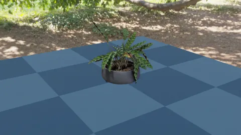
plant.ply Gaussian splat standing on a Genesis World plane, rendered by Nyx under an HDRI environment map. The splat is declared as a LightFieldAsset on the camera rather than as a scene entity, so the environment map only has to light the simulated geometry beside it.Nyx is driven by batched physics rather than scene-by-scene execution, which lets thousands of parallel rollouts run, each with its own scenario, lighting, and camera trajectory, through a single unified pipeline. That coupling is what turns rendering throughput into evaluation throughput, and it is the reason a renderer belongs in a physics platform's story at all.
Quadrants: A Taichi Fork Rebuilt Around Kernel-Orchestration Cost
The same physics pipeline has to run on a robot's onboard computer, on engineers' MacBooks, and on GPU clusters without forking the code per target. Quadrants began as a fork of Taichi in June 2025 — the name is a nod to that origin — and is bundled with Genesis automatically, pinned at quadrants==1.3.0 in the project dependencies. Kernels are written in plain Python and JIT-compiled to NVIDIA CUDA, AMD ROCm, Apple Metal, Vulkan, and x86/ARM64 CPUs via LLVM. Since the fork, the team rebuilt the parts that matter most for simulation workloads and reports up to 4.6x faster runtime on their manipulation and locomotion benchmarks.
The interesting diagnosis is where cost actually lives at simulation scale. It shifts from per-kernel compute to the overhead of orchestrating many small kernels per physics step, and Quadrants attacks that from several angles at once. Each physics step is recorded as a single kernel graph, hardware-accelerated on CUDA (with conditional loops on SM90+) and supported in software on every other backend, which removes launch latency from every top-level loop. Independent kernels overlap through streams instead of serializing through one queue. Where launches do remain, hand-tuned kernel-launch contexts cached at multiple memory tiers keep dispatch overhead sub-microsecond even when many small kernels fire back to back.
Portability is handled by mapping SIMT primitives at the subgroup and block level to each backend's native equivalent — warps of 32 on NVIDIA, waves of 64 on AMD, subgroups on Metal — so a hand-tuned contact solver runs without per-platform branches. Reverse-mode autodiff, previously experimental, is now first-class on every backend, which is what makes differentiable simulation portable across the same hardware policies deploy on. A pure-Python backend was added for debugging and systematic coverage testing.
Inside kernels, dense linear algebra such as Cholesky factorization and triangular solves is expressed in readable Python that compiles to 16x16 tile-blocked code paths, and whole-kernel common-subexpression elimination catches redundant work that block-local optimizers miss. A perf-dispatch layer benchmarks kernel variants on first call for a given argument geometry and caches the fastest choice per signature, so the same frontend code adapts to whatever hardware it runs on. Around all of this sits a three-layer cache for compiled artifacts — compiled kernels on disk plus PTX and fast-cache layers for process startup — which the team credits with a more than 10x startup speedup, cutting startup from minutes to seconds. On the data side, tensors come in two interchangeable types: field for peak runtime throughput and ndarray for fast startup and compile time, switchable at runtime through a unified wrapper. Kernels accept nestable Python dataclasses holding both, and tensors share device memory with PyTorch via DLPack; on Metal, a command queue is shared with PyTorch so zero-copy does not introduce synchronization overhead.
The practical consequence for users is kernel caching behavior you can feel. The first build with a new scene configuration compiles kernels on the fly and is slow; later runs with the same configuration load from cache and start quickly, provided the first run exits normally or via Ctrl-C rather than Ctrl-\.
Sensors, Assets, and a Small API Surface
The simulation interface is where most users actually live. Every Genesis World program starts with one call, gs.init(), which selects the compute backend, fixes numeric precision, seeds the RNGs, and configures logging. Backend resolution for gs.gpu runs in the order CUDA, then AMD, then Metal, then CPU, taking the first that initializes, and falls back to the CPU with a warning rather than failing. Precision is 32-bit by default with precision="64" for stiff or ill-conditioned scenes, though double precision is unavailable on Apple Metal and integer indices are always 32-bit. One knob is worth knowing about: performance_mode=True bakes static tensor shapes into compiled kernels for roughly 30% faster simulation, at the cost of recompiling for several minutes whenever the scene changes. Leave it off for research and interactive work, turn it on for policy training and production runs.
Entities are created from a morph — a combined description of geometry and initial pose — either from primitives (Plane, Box, Cylinder, Sphere, Terrain, Drone) or from files: MJCF, URDF (with .xacro preprocessed automatically), USD in .usd/.usda/.usdc/.usdz, and non-articulated meshes in .obj/.stl/.glb/.gltf with Draco compression supported. Relative paths resolve against both the working directory and the bundled genesis/assets tree, so xml/franka_emika_panda/panda.xml loads the Franka that ships with the project. A URDF base is free by default (MJCF specifies the base joint, URDF does not), which is a real trap until you pass fixed=True.
Sensor coverage is broad and all three renderers are exposed through the same camera-sensor interface. The sensor modules in the tree are camera, depth_camera, imu, raycaster (lidar), contact_force, joint_torque, kinematic_tactile, point_cloud_tactile, probe, surface_distance_probe, and temperature, managed by a sensor_manager. The past year added point-cloud tactile, temperature-grid, and proximity sensors alongside the existing FOTS elastomer-displacement, magnetometer-IMU, and contact-probe suite. Controllers cover control_dofs_position, control_dofs_force, per-DOF kp/kv and force ranges, inverse kinematics (batched), and a Diff-IK controller example. The GUI side ships ImGui joint control, debug drawing, a mesh point selector, and mouse interaction as viewer plugins.
Asset production is treated as its own pipeline. A photogrammetry pipeline turns multi-view captures — collected through an in-house iOS app, a digital camera, or off-the-shelf devices with VIO poses as initialization — into accurate 3D maps, then trains meshes and Gaussian splats end-to-end from the raw images and poses. Both feed Nyx for rendering and Genesis for physics. On top of reconstruction, a programmatic pipeline generates simulation environments including scene layout, asset selection, environment code, and success metrics, so complex environments can be built automatically.
Parallel and Heterogeneous Environments, and What They Measure
A single environment cannot keep a GPU busy, so Genesis World steps many copies of one scene at once. Parallelism is not a property of the entities: you describe the plane and the arm exactly as in the single-environment tutorial, then choose the number of copies at build time.
gs.init(backend=gs.gpu)

scene = gs.Scene(show_viewer=False)
plane = scene.add_entity(gs.morphs.Plane())
franka = scene.add_entity(gs.morphs.MJCF(file="xml/franka_emika_panda/panda.xml"))

# 20 parallel environments; env_spacing only affects viewer layout
B = 20
scene.build(n_envs=B, env_spacing=(1.0, 1.0))

franka.control_dofs_position(
    torch.tile(torch.tensor([0, 0, 0, -1.0, 0, 1.0, 0, 0.02, 0.02], device=gs.device), (B, 1)),
)

# narrow a command to a subset of environments
franka.control_dofs_position(
    torch.zeros(3, 9, device=gs.device),
    envs_idx=torch.tensor([1, 5, 7], device=gs.device),
)
Once n_envs > 0, every per-environment quantity gains a leading batch dimension, documented with the bracket notation ([n_envs,] ...). For the Franka's 9 DOFs, get_dofs_position() returns (20, 9). The envs_idx argument is available on state readers and on all control_dofs_* and set_dofs_* methods, which is the pattern you need when environments finish episodes at different times during training. Tensors should be built on gs.device to avoid host-device copies, the dominant cost at large batch sizes.
The throughput claim is the one people quote, and the benchmark script in the repository is explicit about its conditions. It runs 30,000 parallel environments of a Franka on a plane with performance_mode=True on a GPU backend, and the comment in the source records 43M FPS with the position control applied and 32M FPS without it (the arm then sits in collision with the floor). The docs separately state support for tens of thousands of environments on a single GPU, and the philosophy page claims up to 10-80x the throughput of prior GPU-accelerated simulators such as Isaac Gym/Sim/Lab and MuJoCo MJX, with methodology deferred to the blog post rather than asserted inline.
Heterogeneous simulation goes one step further: different parallel environments can hold different geometry variants of the same entity. Passing a list of morphs to add_entity() distributes variants across environments by balanced block assignment when n_envs >= n_variants (four variants over eight environments puts variants 0-3 in environment pairs), and gives environment i variant i when n_envs < n_variants, leaving the extra variants unused. The example drives all environments through a grasp-and-lift with per-environment IK on objects of different size and shape in one batch.
Scaling out is a second, independent axis, and the guidance is conservative: add a second GPU only once the first is saturated. Genesis World does not split a single scene across GPUs; each process initializes its own runtime, builds its own scene, and runs pinned to exactly one device via CUDA_VISIBLE_DEVICES, QD_VISIBLE_DEVICE (which selects the GPU for Quadrants), and EGL_DEVICE_ID for offscreen rendering — all set before gs.init(). For training, examples/rigid/ddp_multi_gpu.py uses PyTorch DDP with torchrun --standalone --nnodes=1 --nproc_per_node=2, one full scene per rank, seeding Genesis per rank so environments are decorrelated across GPUs. The effective batch is per-GPU n_envs times the number of GPUs. Reinforcement learning plugs in through external libraries: the locomotion example trains a Unitree Go2 with rsl-rl's OnPolicyRunner and PPO (clip 0.2, adaptive KL 0.01, GAE with gamma 0.99 and lambda 0.95, 512-256-128 MLP actor and critic, 24 steps per environment).
Is the Result Trustworthy? The Numbers Behind the Claim
The platform's central claim is about evaluation cost, and it is quantified rather than asserted. A typical model evaluation at Genesis AI runs across hundreds of tasks with each task repeated for hundreds of episodes. In the real world, with one operator and one robot station, a single evaluation pass adds up to more than 200 hours of continuous operation, and statistically meaningful comparisons across checkpoints require many such passes. In simulation, the same tens of thousands of episodes run in less than 0.5 hours — two orders of magnitude faster — require no human or hardware in the loop, and produce bit-exact result consistency across runs.
The bar the team held itself to is zero-shot real-to-sim: policies evaluated in simulation are trained on real-world data only, keeping training and evaluation workflows decoupled. The reason for the separation is methodological. When training and evaluation share the same simulated distribution, an improvement could reflect a genuinely better recipe or merely a tighter fit to the simulator's dynamics. Keeping the pipelines apart gives a cleaner signal about which experiments actually improve model performance.
| Metric | Value | 95% CI | What it means |
|---|---|---|---|
| Pearson correlation (sim vs. real) | 0.8996 | [0.7439, 0.9314] | Simulation tracks real-world performance trends |
| MMRV (Mean Maximum Rank Violation) | 0.0166 | [0.0102, 0.0474] | Simulation preserves the ranking between models |
| FID-based reality gap | 45% smaller | vs. next-best alternative simulator | Rendered images sit closer to the real distribution |
| Wall-clock per evaluation pass | < 0.5 h vs. > 200 h | two orders of magnitude | Evaluation stops being the iteration bottleneck |
The protocol behind those numbers is worth reading carefully, because it is the part that separates a marketing claim from an engineering result. Three models of different scale and architecture (Small, Medium, Large) were evaluated on 14 tasks, with 200 episodes per task, in both the real world and simulation. Correlation metrics were computed with 1,000,000 bootstrap iterations for confidence intervals; each data point is visualized with its bootstrap distribution and 500 sampled regression lines overlaid to show uncertainty in the correlation estimate. MMRV comes from SimplerEnv. The team also notes that open-loop metrics (R-squared and mean absolute error of action prediction on a fixed dataset) did not reflect differences in real-world performance once they fell within a narrow band — open-loop scores catch spikes and serve as a sanity check, but closed-loop metrics are what carry information.
Locating the gaps required instrumentation rather than guesswork. A telemetry system and a real-time side-by-side rig run the simulator and the physical robot in parallel from the same initialization, and the rig lets you choose the source of the policy inputs independently: observations such as camera frames and proprioception can come from the simulator, from the robot, or from a tunable blend of both. Swapping one component at a time and watching where divergence appears attributes the gap to a specific layer — physics, rendering, communication, or control — instead of collapsing everything into a single binary success/failure outcome. The three layers the team tuned were visual fidelity (material properties, lighting models, camera characteristics), robot kinematics and dynamics (joint behavior, friction, contact), and low-level control (faithful replication of the actual on-hardware controller, including timing, latency, and communication characteristics).
Determinism, Replay, and a CLI for Bug Reports
Reproducibility is engineered rather than hoped for. Version 1.3.2 made simulation fully deterministic on a given machine for both CPU and GPU, and 1.3.3 added a torch-like use_deterministic_algorithms option for bit-exact reproducibility. Version 1.4.0 went further: a scene plus a complete trajectory can be exported as a standalone archive that loads on any machine while ensuring bit-exact replay through gs replay, with the stated objective of making bug reports much easier. Scene.export() writes what the scene was authored from and what its build resolved, so the file stands on its own — opening it reads no mesh, model file, or texture from disk. save_checkpoint() writes the scene plus every simulation array, scratch included, as a single-frame .gstraj that load_trajectory() can open.
Export support is scoped honestly: only rigid and kinematic entities carry a description today, and a scene holding anything that alters the simulation (an emitter, a force field) raises and names it, while things a description leaves out (cameras, sensors, per-step callbacks, HDR/EXR textures, runtime visual vertices) are written without plus a warning. The rigid solver also gained contact-handling precision in this period. Version 1.3.1 introduced contact_resolution with a new default, gs.contact_resolution.signorini, which bounds friction against the normal force actually developed by the contact, so normal forces are no longer biased by the friction coefficient or the sliding speed. Version 1.3.3 improved MuJoCo compatibility mode to cover native contact-patch-based multi-contact instead of the older perturbation-based approach, exposed as RigidOptions.enable_contact_patch.
The package installs a gs console entry point with four subcommands: gs launch visualizes an asset (Mesh/URDF/MJCF/USD) with collision-geometry, rotation, scale, and link-frame flags; gs play opens an interactive viewer with ImGui joint controls and simulation; gs replay replays a recorded .gstraj trajectory in the viewer; and gs animate compiles a glob of image files into a video at a given FPS. gs view remains as a deprecated alias of launch.
Engineering Discipline You Can Read in the Repo
Two documents in the repository say more about how the project is maintained than the feature list does. CODING_GUIDELINES.md and the development guidelines file spell out rules that are unusually specific, and several of them are directly about test honesty.
- Never loosen a tolerance to make a failing test pass, and never dismiss a discrepancy as floating-point noise. fp32 rounding is on the order of 1e-6; a drift of 5e-3 on a quantity that should be mathematically exact means a term is dropped or wrong somewhere. Restricting a test's backend or parametrization to sidestep a failure counts as tolerance-widening in disguise.
- Assert physics, not execution. "The simulation runs without error" is not a test. Expected values are derived analytically: free-fall displacement $z = z_0 - \tfrac{1}{2}gt^2$, no ground penetration, velocity decaying to zero at rest, contact stopping a fall.
- Pack tests: one scene build per test. A build recompiles kernels and costs roughly 18 s locally and minutes on CI, so avoiding an extra build is mandatory even at the cost of a harder-to-read test. Batched behavior is parametrized over
n_envs=[0, 2], because multi-env is where shape bugs hide. - Step budgets are hard. Under 100 steps is fine; 100 to 300 needs justification; over 300 is near-prohibited, reserved for four or five tests across the entire suite, and total env-steps are bounded as well since CI cost multiplies every step across the matrix.
- MuJoCo parity as a sanctioned exception.
enable_mujoco_compatibility(off by default) makes the rigid solver reproduce MuJoCo's dynamics to floating-point tolerance, letting Genesis serve as its own baseline: toggling the flag proves a faster replacement integrates to the same state. The mode is for validation, never production, so it must match, never be fast. - Gradient tolerances are pinned to measured floors. Floor $T = \max|\text{ana} - \text{fd}| / (1 + |\text{fd}|)$ at the configured epsilon, worst across CPU and both GPU architectures whose fp32 floors can differ by 4x; tolerance is 1.5x to 5x the floor, with values restricted to {1, 2, 5}e-X. A floor of exactly zero means the check is vacuous, so you fix the loss, not the tolerance.
The code-level rules are equally opinionated and read like scar tissue: getattr/hasattr are prohibited in favor of None initialization and isinstance checks; plain dicts for packing attributes are prohibited in favor of dataclasses or NamedTuples; catch-all exceptions are prohibited except for exception forwarding in multiprocessing; allocations must be exactly sized, with max-size preallocation banned; NaN halts the simulation through the errno mechanism because a warning is not acceptable; legacy and deprecation layers get removed rather than carried; and domain nouns are restricted to entity, link, and geom — never invent "body", "object", or "piece" when one of those fits, which doubles as a correctness cue since the rigid-body unit is the link. Kernel signatures follow a canonical parameter order (indices, then dynamic scalars and fixed-size vectors, then tensors, then state structs, then info structs, then static configs, then compile-time flags, with errno last).
The test suite mirrors that structure: folders per component (rigid/ with 18 files, sensors/ 10, grad/ 9, core/ 8, rendering/ 8, ipc/ 5, particles/ 5, parsers/ 4, coupling/ 3, deformable/ 3, plus benchmarks/ and integration/), one file per capability, and new coverage added to the test that already covers it rather than a sibling function. Bug-fix PRs must include a regression test that fails on main and passes with the fix. Dependencies are pinned with reasons written inline — MuJoCo is constrained to >=3.10.0,<3.11.0 in dev because 3.10.0 aligned the primal solvers with Genesis (Hager-Zhang CG update, shifted linesearch costs), and step-by-step solver consistency tests only hold when both engines run the same algorithm.
Install, Extras, and Where It Is Headed
Installation is one command after PyTorch: pip install genesis-world for Python 3.10 to 3.13, or pip install -e ".[dev]" from a clone for contributors, which the docs recommend re-running after every HEAD move so dependencies and entry points stay current. uv sync works too. Two extras are optional: pip install pyuipc for the IPC solver backend (Linux / Windows x86, NVIDIA GPU) and pip install gs-nyx for the Nyx renderer. Quadrants is bundled automatically; a standalone pip install quadrants wheel exists for users who want the compiler outside Genesis.
The catalogue of 122 examples is organized to mirror the layers: physics (37 rigid, 12 coupling, 6 IPC, 5 SAP coupling, 5 deformable, 5 collision, 2 fluid), rendering (6 in-repo camera setups plus the Nyx walkthroughs hosted in the genesis-nyx repository), and simulation interface (11 sensors, 9 drone, 7 locomotion, 5 manipulation, 4 viewer plugins, 2 GUI, 4 speed benchmarks). Most run end-to-end after an editable install; the IPC and Nyx examples need their extras.
Three directions are stated for what comes next. First, scaling post-training by scaling simulation environments: closed-loop evaluation becomes a data engine for exploration where the model attempts tasks, fails, is scored, and improves across millions of iterations and thousands of parallel tasks, with the simulator acting as both environment and critic — the same playbook large-scale RL followed in LLM development. Second, a hybrid simulator. Genesis World today is classical and heuristic, which gives full controllability and observability over every layer: every knob is explicit and every behavior can be inspected, modified, and attributed. Learned simulators progress quickly but much of their state remains implicit and ungrounded, which is where classical simulators are still stronger. The plan is to merge the two in a data-driven way, with classical simulation bringing grounding and learned world models bringing scale and realism. Third, self-evolving physical AI as the north star: an inner loop in simulation where agents generate environments, the model acts, the simulator scores, and the policy improves, and an outer loop in the real world where deployments surface edge cases that recalibrate the simulator and get folded back into the task distribution. Every variable a researcher would normally touch — data mixture, architecture, reward, curriculum, new environments — becomes tunable by agents as long as each change is verifiable.
The license is Apache 2.0, and the acknowledgments name the projects the work stands on: Taichi, which Quadrants forked from; libuipc for the IPC backend; FluidLab and SPH_Taichi as reference MPM and SPH implementations; Ten Minute Physics and PBF3D for PBD; MuJoCo for rigid body dynamics and libccd for collision detection; PyRender for rasterization; LuisaCompute and LuisaRender for the ray-tracing DSL; and Madrona and Madrona-mjx as the batch renderer backend. Two citations are offered: the May 2026 Genesis AI blog post for Genesis World 1.0, and the original December 2024 Genesis entry for the academic project it grew out of.