PAPER DEEP DIVE
GeoFlow-SLAM: A Robust Tightly-Coupled RGBD-Inertial and Legged Odometry Fusion SLAM for Dynamic Legged Robotics
GeoFlow-SLAM targets the feature-matching, initialization, and texture-robustness failures that arise when legged robots move aggressively at high frequency. It tightly couples dual-stream optical flow, legged odometry, PnP, GICP, and depth-to-map geometric constraints in one optimization framework. Experiments on Unitree Go2 and G1 robots plus OpenLORIS, ScanNet, and TUM datasets show state-of-the-art robustness and accuracy.
Paper information: Tingyang Xiao, Xiaolin Zhou, Liu Liu, Wei Sui, Wei Feng, Jiaxiong Qiu, Xinjie Wang, and Zhizhong Su, March 18, 2025, accepted to IROS 2025. Paper: https://arxiv.org/abs/2503.14247. Code: https://github.com/HorizonRobotics/GeoFlowSlam, publicly released.
One-sentence summary: GeoFlow-SLAM places dual-stream optical flow, legged odometry, GICP, and depth-to-map constraints in a single factor graph, keeping legged-robot localization stable during aggressive motion and texture-poor navigation.
1. Why ordinary visual SLAM fails on legged robots
An RGB-D camera supplies both color and depth in one exposure, which is attractive for robot SLAM. A legged platform, however, is not a smooth camera mount. Acceleration, posture changes, and high-frequency body vibration introduce motion blur and abrupt inter-frame displacement. ORB features that are dependable in textured static scenes can therefore be projected into the wrong image neighborhood, sharply reducing the number of inliers.
The second failure is initialization. Conventional visual SLAM often uses a constant-velocity model or IMU pre-integration to predict the current pose. On a legged robot, each gait cycle changes speed and body morphology, producing non-smooth excitation. IMU pre-integration may drift away from the true motion over a short interval. Once the initial pose is wrong, the subsequent optical-flow search, depth association, and local optimization can converge in the wrong basin.
The third failure is texture deficiency. Offices, corridors, and structured interiors often contain large white walls, repetitive patterns, and surfaces with few corners. When visual observations are scarce, reprojection factors alone do not contain enough geometric information to recover the pose. The depth image still observes planes and structures, but registering a full point cloud against the map for every frame is computationally expensive.
GeoFlow-SLAM therefore does not merely stack sensors. It assigns complementary roles: optical flow handles feature correspondence during fast motion, legged odometry and GICP stabilize initialization, and depth-plane constraints supply geometric support when vision weakens.
2. System overview: a pipeline designed around degradation modes
The input stream consists of RGB images, depth maps, IMU measurements, and legged odometry. The tracking thread first predicts the current pose from the available sources, then establishes feature correspondences through dual-stream optical flow. It constructs visual reprojection, IMU pre-integration, GICP relative-pose, and depth-to-map factors. Local keyframe optimization jointly estimates the poses and map points in the window. To control computation, depth-to-map constraints are added to a frame node only when valid visual observations are insufficient.
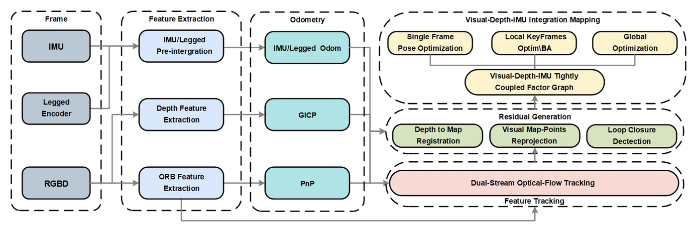
The essential design change is that initialization, matching, and optimization are not isolated. Optical flow consumes a prior pose supplied by IMU, legged odometry, PnP, or GICP; the optimized state then updates the map and local geometry that will guide the next projection. This feedback loop prevents a single degraded observation from immediately causing runaway drift.
3. Dual-stream optical flow: let the map explain the current image first
The first stream is 3D-to-2D optical flow. Let $P(X,Y,Z)$ be the map point associated with a previous feature and $T_{wk}^{c}$ be the initial pose. The point is projected into the current frame as:
$$p'(x,y)=F(T_{wk}^{c}P)$$The camera projection model is:
$$F(P)=\begin{bmatrix}f_X\frac{X}{Z}+c_x\\f_Y\frac{Y}{Z}+c_y\end{bmatrix}$$The projection is not treated as the final match. Instead, optical flow starts from this geometrically plausible location and searches in the current image. The search remains near a pose-consistent region instead of blindly seeking the nearest descriptor under large displacement.
The second stream handles previous-frame features without a qualified map-point association. These points are tracked between the previous and current images, then merged with the first stream. The first stream has an explicit scale and is less sensitive to appearance changes; the second stream preserves short-term image motion without requiring an existing map point. The paper calls the combined mechanism GeoFlow.
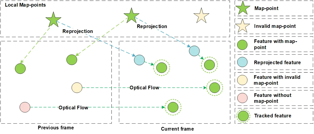
The value of this split is that failures do not propagate unchecked. If the IMU or odometry prior is slightly wrong, map-point reprojection can still land close to the correct feature. If some features have no map association, the second stream can still maintain short-term continuity. Together they give the backend enough observations to avoid an erroneous local minimum.
4. Initialization: legged odometry first, then PnP and GICP
The authors explicitly prioritize legged odometry when it is available, avoiding initial poses distorted by legged-robot IMU error. An IMU remains useful over short durations and is computationally simple, so it is also an appropriate prediction source. If those sources are unavailable or fail, the system computes an essential matrix from successfully tracked features and recovers frame-to-frame motion. Because that recovery lacks scale, PnP is then performed using depth to obtain a scaled initial pose. If PnP fails, GICP refines the pose; only when all preceding methods fail does the system fall back to the constant-velocity model.
This order reflects a practical engineering judgment. Kinematic odometry on a legged robot is not global truth, but within a gait cycle it can be more stable than an IMU affected by vibration. GICP can exploit geometric structure when vision degenerates. The open-source `Tracking.cc` implements this sequence in `TrackWithMotionModelICP()`: it predicts state with IMU or optical flow, calls `PredictStateOdom()` when robot odometry is available, invokes `PredictStateICP()`, and then runs `SearchByProjectionWithOF()`.
5. The local factor graph: four residual families constrain the state
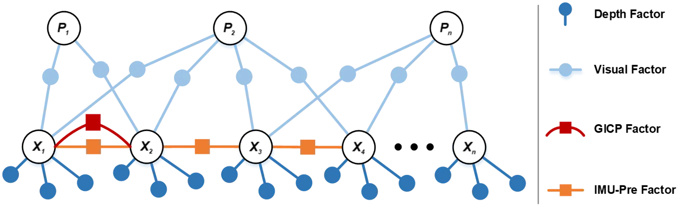
In local keyframe optimization, GeoFlow-SLAM jointly estimates window poses $x_1,\ldots,x_n$ and map points $P_1,\ldots,P_n$. The paper writes the objective as four robust residual groups:
$$r_1=\min_{X}\sum_{(i,j)\in F}\rho\left(\|r_v(p_i^c,X)\|_{\Sigma_v}^2\right)$$$$r_2=\min_{X}\sum_{i\in F}\rho\left(r_{imu}^T\left(z_{b_i b_{i+1}}^c,X\right)\Sigma_{b_i b_{i+1}}^{-1}r_{imu}\left(z_{b_i b_{i+1}}^c,X\right)\right)$$
$$r_3=\min_{X}\sum_{(i,j)\in F}\rho\left(r_{gicp}^T\left(I_{j i}^c,X\right)\Sigma_{gicp}^{-1}r_{gicp}\left(I_{j i}^c,X\right)\right)$$
$$r_4=\min_{X}\sum_{(i,j)\in F}\rho\left(\|r_l(d_i^c,X)\|_{\Sigma_l}^2\right)$$
Here $r_1$ is the visual reprojection residual, $r_2$ the IMU pre-integration residual, $r_3$ the GICP relative-pose residual, and $r_4$ the depth-to-map residual. Covariance matrices encode observation uncertainty, while $\rho$ is a robust kernel that suppresses incorrect matches and point-cloud outliers. In local bundle adjustment, $X$ includes the IMU states and map points; in single-frame optimization, it contains only adjacent-frame IMU states.
6. Depth-plane features and point-to-plane residuals
To avoid the cost of direct full depth registration, the system first extracts plane features from depth point clouds. Following a strategy similar to SSL-SLAM, it computes vertical and horizontal angles for each point:
$$\alpha_i=\arctan\left(\frac{z_i}{\sqrt{x_i^2+y_i^2}}\right)$$$$\theta_i=\arctan\left(\frac{y_i}{x_i}\right)$$
These angles partition the detection range into $M\times N$ cells. The method computes a geometric center in each cell and evaluates local smoothness; lower smoothness indicates a plane-like feature. Depth-plane points from keyframes are then stitched into a local map. For a plane point in the current keyframe, the method projects it into the local map and fits a plane to its k nearest neighbors, producing a point-to-plane constraint.
The residual is:
$$r_l(d_i^c,X)=(n^w)^T\left(P'-q_{plane}^w\right)=JX+\omega$$with Jacobian:
$$J=\frac{\partial r_l}{\partial X}=\frac{\partial r_l}{\partial P'}\frac{\partial P'}{\partial X}=(n^w)^T[I,-P'^\wedge]$$and transformed point:
$$P'=T_{cw}^c p_{plane}^c$$$n^w$ is the plane normal in the world frame, $q_{plane}^w$ is the plane center, $p_{plane}^c$ is the plane point in the camera frame, and $\omega$ is observation noise. The residual does not require a point to coincide with a particular map point; it requires the point to lie on the observed plane, which is well suited to walls, floors, and tabletops.
7. Correspondence with the open-source implementation
The repository contains verifiable core code rather than only figures. In `src/Tracking.cc`, `TrackWithMotionModelICP()` forms the pose prior through IMU, optical flow, robot odometry, and GICP. When `UseOpticalFlow` is enabled, it invokes `SearchByProjectionWithOF()`. If fewer than 25 matches are found, it adds features and repeats the flow search with a wider window and half the distance threshold.
`src/RegistrationGICP.cc` wraps GICP in `RegisterPointClouds()`, using four threads, a 0.02-meter downsampling resolution, and a 0.1-meter maximum correspondence distance before calling `small_gicp`'s `align()`. In `src/Optimizer.cc`, local keyframe optimization calls `RegisterPointClouds()` to estimate the relative pose between adjacent keyframes and inserts it as a Sim3 edge. For keyframes with no more than 75 matching inliers, `GenerateLidarEdge()` creates point-to-plane edges with information weight 100 and a Huber robust kernel. These implementation points correspond directly to the equations and pipeline in the paper.
8. Experimental setup and Go2/G1 results
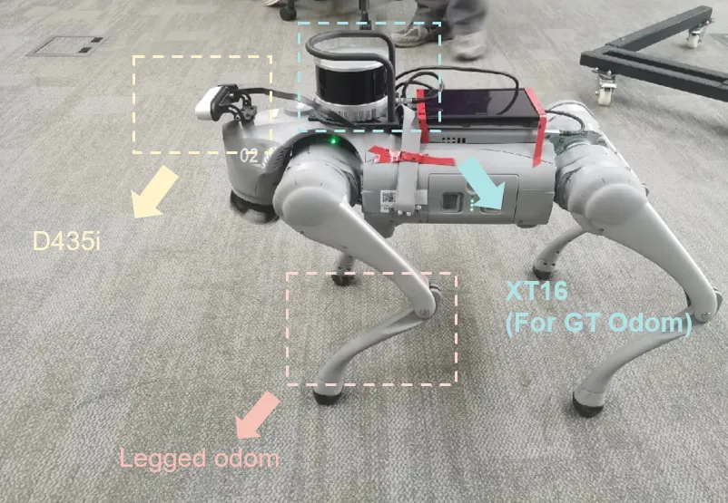
The authors evaluate on a Unitree Go2 quadruped and a G1 humanoid. Go2 carries a D435i camera at approximately 10–15 FPS, a Bosch BMI055 IMU at about 200 FPS, an XT16 LiDAR at about 10 FPS, and a legged-odometry system at about 500 FPS. G1 carries a D435i at about 25–30 FPS, a Mid360 LiDAR at about 10 FPS, and legged odometry at about 500 FPS. Ground truth comes from an enhanced LIOSAM system for legged robots; LIO-SAM and legged-odometry trajectories are aligned to estimate the IMU-to-legged-odometry extrinsic.
The following table reports ATE in meters on the Go2 D435i dataset. A slash denotes tracking failure.
| Sequence | VINS-RGBD | S-VIO | ORB-SLAM3 | GeoFlow-SLAM |
|---|---|---|---|---|
| Seq1 | 0.8316 | 1.3621 | failed | 0.0947 |
| Seq2 | failed | failed | failed | 0.1369 |
| Seq3 | failed | failed | failed | 0.6009 |
| Seq4 | failed | failed | failed | 0.4458 |
| Seq5 | 0.3223 | 0.7121 | 0.2963 | 0.1709 |
| Seq6 | failed | failed | failed | 0.6235 |
On Seq1, GeoFlow-SLAM improves over VINS-RGBD by about 88% and over S-VIO by about 93%. More importantly, most baselines fail on Seq2, Seq3, Seq4, and Seq6, whereas GeoFlow-SLAM completes tracking. The reported average per-frame runtime on an i9-13900H is 20.1–27.6 milliseconds, indicating that the robustness gain does not completely sacrifice real-time operation.
9. OpenLORIS results
OpenLORIS contains dynamic home and office environments. The paper compares VINS-Mono, VINS-RGBD, ORB-SLAM3, S-VIO, VID-SLAM, DDIO-VIO, and GeoFlow-SLAM. The table below selects the Office sequences plus Home1-1; ATE is again in meters.
| Sequence | VINS-Mono | VINS-RGBD | ORB-SLAM3 | S-VIO | GeoFlow-SLAM |
|---|---|---|---|---|---|
| Home1-1 | 1.0760 | 0.4520 | 0.9290 | 0.4020 | 0.4575 |
| Office1-1 | 0.2310 | 0.1010 | 0.0680 | 0.1010 | 0.0577 |
| Office1-2 | 0.2890 | 0.1240 | 0.1230 | 0.0990 | 0.0700 |
| Office1-3 | 0.1550 | 0.1540 | failed | 0.1510 | 0.0291 |
| Office1-4 | 0.3920 | 0.1860 | 0.2530 | 0.1640 | 0.1554 |
| Office1-5 | 0.2380 | 0.2390 | failed | 0.2120 | 0.2000 |
The method is not uniformly first. On Home1-1, S-VIO reaches 0.4020 meters, better than GeoFlow-SLAM's 0.4575 meters; on Office1-4, S-VIO's 0.1640 meters is slightly better than 0.1554 meters. GeoFlow-SLAM nevertheless achieves the lowest or near-lowest error on most Office sequences and maintains a stronger completion rate on the critical sequences. For a legged robot, the gap between failure and success often matters more than a few centimeters between two successful trajectories.
10. Ablation: what each module contributes
The ScanNet ablation uses sequences 50, 59, 84, 106, 169, 181, 207, 580, and 616. The TUM ablation uses a long office sequence plus multiple low-texture and low-structure sequences. Four configurations are compared: r+o adds optical flow, r+i adds GICP, r+d adds depth-to-map constraints, and r+o+i+d is the complete system. All runs use RGB-D mode without IMU or legged odometry.
| Dataset | Metric | ORB-SLAM3 | r+o | r+i | r+d | r+o+i+d |
|---|---|---|---|---|---|---|
| ScanNet | ATE | 0.2638 | 0.2404 | 0.1055 | 0.0775 | 0.0779 |
| ScanNet | RTE | 0.0101 | 0.0095 | 0.0100 | 0.0094 | 0.0090 |
| TUM | ATE | 0.0341 | 0.0142 | 0.0156 | 0.0155 | 0.0129 |
| TUM | RTE | 0.0136 | 0.0089 | 0.0106 | 0.0100 | 0.0086 |
On ScanNet, the complete system's mean ATE is 0.0779 meters, about 70% better than ORB-SLAM3's 0.2638 meters. On TUM, the complete system achieves 0.0129-meter ATE and 0.0086-meter RTE, improvements of approximately 62.2% and 36.7%. ORB-SLAM3 fails on ScanNet sequences 50, 84, 181, 207, and 616 and on TUM sequences str_notex_far, str_notex_near, and nostr_tex_far; all four GeoFlow configurations complete every sequence.
The ablation also reveals complementarity. On ScanNet, r+d alone reaches 0.0775 meters, slightly better than the full system's 0.0779 meters, showing that depth-plane constraints are already powerful in structured interiors. On TUM, r+o alone reduces ATE from 0.0341 to 0.0142 meters, showing the importance of optical flow for fast-motion matching. The full system's advantage is cross-scene stability rather than mechanically minimizing every individual number.
11. Extremely hard scenes and comparison with STL-SLAM
On TUM's no_structure_notexture_far and nostructure_notexture_near scenes, GeoFlow-SLAM obtains ATE values of 0.0308 and 0.0467 meters. The authors argue that repetitive texture and sparse features can mislead conventional optical flow, while GeoFlow uses a more accurate pose prior to restrict the search. When visual observations are absent, depth point-to-plane and GICP relative-pose factors continue to constrain the optimization and prevent divergence.
The comparison with STL-SLAM is favorable but not universal. On fr1/xyz, STL-SLAM reaches 0.0100 meters while GeoFlow-SLAM reaches 0.0101 meters. On fr3/str_notex_near and fr3/str_tex_near, ORB-SLAM3 is slightly better at 0.0126 and 0.0093 meters versus 0.0126 and 0.0094 meters. On fr3/cabinet and fr3/large_cabinet, ORB-SLAM3 fails while GeoFlow-SLAM reaches 0.0500 and 0.0601 meters. The benefit is robust completion, not unconditional superiority on every ordinary sequence.
12. Limitations
First, the experiments rely on substantial compute. Although 20–27.6 milliseconds per frame on an i9-13900H is close to real time, that does not guarantee direct deployment on a low-power onboard computer. GICP, plane extraction, and point-to-plane edge generation add overhead and may require pruning for embedded robots.
Second, the geometric constraints assume reliable planes or structures in the local map. In an environment that is both texture-poor and structure-poor, depth-to-map constraints become less informative. The paper demonstrates extreme low-texture scenes, but completely unstructured settings still deserve more evaluation.
Third, ground truth is generated by an enhanced LIOSAM system, and trajectory alignment is used to estimate the extrinsic between the IMU and legged odometry. This setup is reasonable, but the quality of ground truth and calibration can affect interpretation of absolute errors, especially for small differences.
Fourth, GeoFlow-SLAM is not best on every successful OpenLORIS or TUM sequence. S-VIO, STL-SLAM, or ORB-SLAM3 can achieve lower ATE on some sequences. The system's strength is completion under aggressive legged motion and degraded observations, not a blanket replacement for every RGB-D or VIO method.
13. Method diagram
This diagram captures the branch that distinguishes GeoFlow-SLAM from ordinary visual SLAM: geometric depth constraints are not always on; they are triggered when visual observations become insufficient.
14. Conclusion
GeoFlow-SLAM makes three concrete contributions. It brings map points and pose priors into optical flow so that fast-motion matching has a geometric boundary. It builds a legged-odometry, PnP, and GICP initialization cascade that reduces the effect of IMU error on legged robots. Finally, it tightly couples visual reprojection, IMU pre-integration, GICP relative pose, and depth point-to-plane residuals in a local factor graph, so texture-poor scenes retain geometric constraints.
The engineering significance is that the paper makes each recovery path explicit: where the initial pose comes from, how the search window is bounded, when geometric factors intervene, and how the optimized state feeds back into the next frame. The public implementation confirms that these mechanisms are present, making the system practical to port and adapt.
Golden sentence: When vision degrades, a robot does not need more pixels; it needs geometric constraints that still hold.