ReST-RL: Reinforcing LLM Reasoning through Unified Self-Training and Value-Guided Search

Paper: ReST-RL: Reinforcing LLM Reasoning through Unified Self-Training and Value-Guided Search (arXiv:2508.19576v3, 29 pages, revised 2026-09-07)
Authors: Sining Zhoubian (Tsinghua University; work done while interning at Z.ai), Dan Zhang (Department of Computer Science and Technology, Tsinghua University), Jie Tang (Department of Computer Science and Technology, Tsinghua University)
Code: released at GitHub THUDM/ReST-RL (commit b86959b verified for this write-up), covering MCTS, GRPO training, value-model training and the evaluation harness
Subject: reinforcement learning for LLM reasoning plus value-guided decoding at inference time. The primary empirical domain is code generation, with out-of-domain transfer evidence on math and science.

One-Sentence Summary

ReST-RL splits the "GRPO rewards carry too little information" problem into two separately tractable pieces: stage one, ReST-GRPO, filters prompts by reward standard deviation and draws prefixes from high-reward trajectories under a discrete exponential distribution to serve as fresh starting contexts for online RL, thereby reshaping the policy-induced trajectory distribution; stage two, VM-MCTS, runs MCTS under the now-static policy to self-collect value targets and trains a value model that predicts expected terminal reward, letting one and the same model allocate the inference-time search and rank the final candidates. On six coding benchmarks Qwen3-8B moves from 0.503 to 0.689 average.

Background and Motivation

GRPO has become the representative RL method for raising LLM reasoning accuracy. It removes the explicit value network and replaces it with a relative reward difference computed inside a sampled group, so its training cost is far below that of PPO-style online actor-critic. The price is that reward learning is taken out of the RL loop entirely: a whole trajectory yields a single scalar at its terminal state, and the group-relative advantage depends completely on how much those rewards differ from one another. The paper's first diagnosed weakness sits exactly here. When the solutions sampled for one prompt receive similar rewards, the group-relative advantage degrades into noise and that update carries almost no information; Figure 1(a) of the paper gives the direct statistic for this phenomenon. DAPO mitigates it through dynamic sampling, repeatedly re-drawing until enough groups with non-zero reward variance are retained, together with a decoupled clipping upper bound and truncation masking. The other route is a prompt-level curriculum such as the cosine schedule of E2H Reasoner, which shifts training from easy to hard questions over time.

The paper's criticism of both remedies is precise: they still operate at the level of the original prompt. Dynamic sampling changes which groups survive; a curriculum changes which questions are presented. Neither goes back inside a trajectory that already succeeded to re-use the intermediate states that plainly carry information. In other words they optimize what to ask, not where within a solution to resume asking.

The second weakness is on the verification side. Process reward models score intermediate steps and generally verify more accurately than outcome reward models that only look at the final output, but they depend on high-quality human step annotation. Collecting a corpus of the PRM800K kind is famously expensive, which caps scalability. To dodge annotation, Math-Shepherd and ReST-MCTS* estimate process rewards with Monte-Carlo simulation instead: roll out several times from a given intermediate step, measure how often the final answer is correct, and treat that proportion as the "correctness" of the step. The trouble is that this estimate is welded to task-specific answer matching and to a fixed notion of step correctness. Coding fails on both counts. A single intermediate line is neither correct nor incorrect on its own, and a solution that passes its tests can be built out of lines that look odd in isolation; yet a complete solution can be scored automatically by test cases.

The paper therefore frames the state of the art as a three-way trade-off among data-collection cost, informative policy updates, and fine-grained inference-time guidance, with existing methods capturing at most two of the three. Its design goal is correspondingly modest: keep GRPO's lightweight policy update while recovering state-level learning signals, and do so without returning to the full cost and instability of online actor-critic learning.

One methodological point deserves separate mention because it determines how the experiments should be read. The paper explicitly separates two roles that are routinely conflated: improving the policy's training distribution, and learning a value signal for allocating inference-time compute. It then concedes that connecting the two only counts as established under one condition: the first-stage policy improvement must survive a matched value-learning pipeline, rather than merely producing a better policy-only checkpoint. That sentence maps onto Table 3(b) in the experiments, which is the most convincing controlled comparison in the paper.

Preliminaries: How the Task Is Turned Into an MDP

A reasoning task is described by an instruction or question $q$; a ground-truth answer $g$ may exist, and for coding tasks there may additionally be test cases $t_{1,2,\dots,m}$. The policy $\pi_{\theta}$ generates a solution step by step following its predicted output token probabilities, and the process is modelled as a Markov process: the policy takes action $a_i$ according to $\pi_{\theta}(a_i|a_{1,2,\dots,i-1},q)$, conditioned on the previously generated content and the instruction, until an eos token or a stop string is produced, forming the final solution $A=(a_1,a_2,\dots,a_k)$.

The granularity choice for an action in this paper is a single line of text, delimited by a line break. An intermediate state is defined as the combination of the instruction and a partial solution, $S_i=(q,a_{1,2,\dots,i})$, so an intermediate state always terminates with a line break; an end state is $S_{end}=S_k=(q,a_{1,2,\dots,k})$, terminating with eos. Transitions are treated as deterministic. Appendix A.8 justifies the granularity: relative to token-level actions, line-level actions substantially reduce the branching complexity of tree search and make value estimation more stable, since each transition corresponds to a semantically more meaningful unit; relative to coarser alternatives such as a whole reasoning step or a whole code block, line-level actions need no domain-specific segmentation rules and no extra annotation, so they transfer across domains unchanged. The paper does not claim this granularity is universally optimal and lists adaptive or task-specific action abstractions as an open direction.

Rewards are assigned only to end states, written $R=R(S_{end})$, and may be rule-based or model-based. Under this setup the policy value function and the Q function collapse into the same quantity:

$$V^{\pi}(S_i)=\mathbb{E}_{\pi}[R(S_{end})|S_i],\qquad Q^{\pi}(S_i,a_{i+1})=\mathbb{E}_{\pi}[R(S_{end})|S_{i+1}]=V^{\pi}(S_{i+1})$$

This is Equation 1 and it is the foundation of everything that follows. Because only end states carry reward and transitions are deterministic, "the value of state $S_i$" and "the value of taking action $a_{i+1}$ in $S_i$" are the same expectation under different conditioning. The value model therefore needs no separate Q head: learning $V^{\pi}$ suffices, and the estimate of a child node during search is already its Q value.

Method

Overall Framework: Sequential Connection, Not Joint Optimization

ReST-RL has two components: the policy-optimization stage ReST-GRPO and the reward-learning stage VM-MCTS. What matters is that the connection between them is sequential. ReST-GRPO first reshapes the trajectory distribution over a sparse reward space; VM-MCTS then estimates values under the resulting static policy. That separation recovers state-level guidance while avoiding the cost and instability of online actor-critic learning. Because $V^{\pi}$ is itself policy-dependent, the paper insists that each value model be paired with the policy that generated its training trajectories. The matched comparison in Table 3(b) is designed on exactly this principle and introduces no policy-value mismatch.

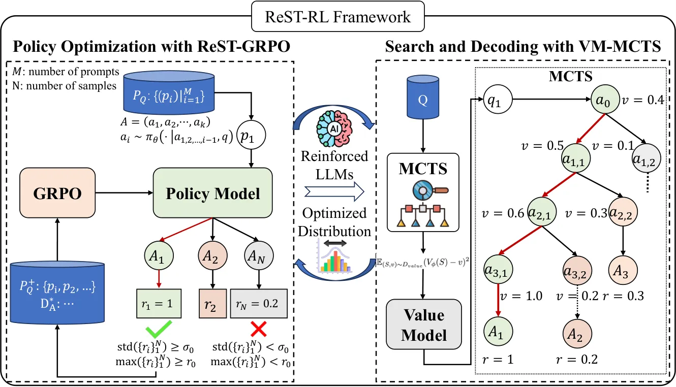
Figure 1: The ReST-RL framework (paper Figure 2). ReST-GRPO reshapes the policy-induced trajectory distribution by filtering and assembling high-value training data; the improved distribution improves value-model learning, which in turn lets VM-MCTS perform more reliable value-guided search and decoding.

ReST-GRPO: A Prefix Is Context, Not an Imitation Target

ReST-GRPO adds two moves on top of ReST and GRPO: reward-based filtering, and starting from partial states. There is one distinction from classical ReST-style self-training that must be stated plainly. Classical ReST and ReST^EM fit the accepted complete completions as a supervised target. ReST-GRPO uses an accepted prefix only as context; its suffix is freshly sampled online and optimized with the GRPO objective. The stored trajectory therefore determines where online RL may restart, and does not prescribe what the policy should generate afterwards. This is the dividing line between the present work and the whole family of "imitate the high-reward solution" methods, and it is why the diversity experiment in Table 19 shows no mode collapse.

Each iteration has three steps. The complete procedure is Algorithm 1 of the paper, with detailed pseudocode in Appendix Algorithm 2; every iteration is initialized from the checkpoint produced by the previous round.

Step 1, pre-train solution sampling. For every instruction prompt in the source dataset, $N$ solutions are collected with the current policy ($N=30$ by default). The sampling temperature controls the randomness and diversity of those solutions, and a fixed reward function then scores all of them for the subsequent filtering.

Step 2, data filtering by reward. The paper derives three observations from the fact that GRPO's update relies on group-relative advantage. First, if a policy's outputs obtain similar rewards on a question, there is little for it to learn there. Second, for questions where the action space is enormous but only a few traces reach a substantial reward, ordinary sampling from the initial state is ineffective for training. Third, for a question the current policy handles poorly, high-reward traces are crucial; and since high-reward solutions often share common patterns, sampling from a partial state of a high-reward solution is more likely to yield further high-reward traces.

The corresponding filter is two gates. The first uses standard deviation to measure reward variety: a prompt whose sampled rewards have standard deviation below the threshold $\sigma_0$ (default 0.05) is dropped from the training set because it will plausibly produce very little policy improvement, while prompts that pass are added together with their original prompt. The second gate concerns high-reward anchors: prompts whose best reward still falls below $r_0$ (default 0.9) are discarded, and for the rest the highest-reward trace is extracted as $A^{*}=\arg\max_{A_i}r_i$.

Step 3, train-data assembly. A subset $D_A^{*}$ of the partial states of $A^{*}$ is drawn from a discrete finite exponential distribution with a fixed positive exponent factor $\alpha<1.0$ (default 0.95):

$$p(a_{1,2,\dots,j})=\frac{1-\alpha}{1-\alpha^{|A|}}\alpha^{j-1},\qquad j=1,2,\dots,|A|$$

This is Equation 2. Relative to uniform sampling it places more mass on shorter, earlier prefixes, which retains a larger suffix action space for online exploration. In total $\beta|A|$ partial states are sampled ($\beta=0.5$ by default, bounding the training budget), each appended to the initial prompt $p$. The paper flags one degenerate case worth noting: as $\alpha\to 0$ the mass concentrates on the shortest prefix, so the resulting starts approach ordinary GRPO-style starts but are not identical to using only the original prompt. That is an easy detail to misread.

Step 4, GRPO training. The update uses the standard GRPO objective; the only difference is that the policy's input prompt may be a combination of the question and a sampled partial solution, drawn from the assembled set $P_Q^{+}$:

$$\mathcal{J}(\theta)=\mathbb{E}\big[p\sim P_Q^{+},\{o_i\}_{i=1}^{G}\sim\pi_{\theta_{old}}(O|p)\big]\frac{1}{G}\sum_{i=1}^{G}\frac{1}{|o_i|}\sum_{t=1}^{|o_i|}\Big\{\min\big[\frac{\pi_{\theta}(o_{i,t}|p,o_{i,<t})}{\pi_{\theta_{old}}(o_{i,t}|p,o_{i,<t})}\hat{A}_{i,t},\ \mathrm{clip}\big(\frac{\pi_{\theta}(o_{i,t}|p,o_{i,<t})}{\pi_{\theta_{old}}(o_{i,t}|p,o_{i,<t})},1-\epsilon,1+\epsilon\big)\hat{A}_{i,t}\big]-\beta^{\prime}\mathbb{D}_{KL}[\pi_{\theta}||\pi_{ref}]\Big\}$$

This is Equation 3. The rollout group size is $G=8$ and all policy methods use a learning rate of 1e-7. The training reward adds two shaping terms on top of test-case pass rate (Equation 7), with weights $\omega_1=1\mathrm{e}{-3}$ and $\omega_2=1\mathrm{e}{-6}$:

$$R_{\text{GRPO}}(q,A)=R_{\text{base}}(q,A)+\omega_1\cdot\mathbb{I}(s\subseteq A)-\omega_2\cdot n\_redundant\_char(A)$$

Here $s$ is a required output substring and the second term penalizes redundant characters. The naive GRPO baseline is trained with the same $R_{\text{GRPO}}$; the only difference is the training data, since the baseline uses the questions of $Q_{\text{train}}$ directly and each question is used once per training iteration.

VM-MCTS: Replacing "Step Correctness" with Expected Terminal Reward

VM-MCTS trains a value model from self-collected MCTS targets under a static policy and uses it for inference-time search and selection. Its target is the expected terminal reward $V^{\pi}(s)$ of a partial state, not whether the most recent line is independently correct. The distinction matters in executable-reward settings, where intermediate steps are hard to label even though complete solutions can be evaluated automatically. The value model plays two roles: allocating search toward promising reasoning subspaces, and ranking completed candidates.

The relationship to Math-Shepherd is stated cleanly. In M-S the quality of an intermediate step is defined as its potential to deduce the correct final answer, which is already an expectation-based evaluation target; but M-S still treats that estimate as a measure of single-step correctness. VM-MCTS instead subsumes it under the value target of Equation 1, emphasizing evaluation of the whole partial state including the last action. In fact the M-S soft target is a special case of the value target, obtained when the reward function takes the answer-matching form

$$R(S_{end})=\mathbb{I}(a_A=a^{*}),\qquad s.t.\ \ S_{end}=(q,A)$$

that is, Equation 4. Conversely, for coding one swaps $R$ for test-case pass rate and the same value-learning machinery applies unchanged, which is precisely why the approach lands in the code domain.

Value-data collection. MCTS is used to collect the value model's training data (Algorithm 3), because it balances exploration of different reasoning paths against exploitation of promising intermediate states. The root of the search tree is the initial state $S_{init}=S_0=(q,\varnothing)$ and other nodes represent intermediate or end states. Node selection uses UCT:

$$S\leftarrow\arg\max_{S^{\prime}\in\text{children}(S)}\left(v_{S^{\prime}}+c\sqrt{\frac{\ln N_S+1}{N_{S^{\prime}}+\epsilon}}\right)$$

where $c$ is the exploration constant (0.4 during collection, 0.1 for test-time decoding), $\epsilon=0.1$ avoids division by zero, $N$ is the visit count and $v$ the current mean value estimate. During expansion the algorithm samples $n=5$ traces from $S$ and builds child nodes from the first action of each trace. It then performs a full MC rollout, scoring those $n$ complete traces with the reward function and writing the resulting end-state value targets into $D_{value}$; values are backpropagated along the path, updating visit counts $N$, reward sums $U$, and $v=U/N$. The search runs for $T=30$ iterations (main results and matched controls use $T=20$). Unlike the all-at-once estimation of M-S, partial-state values here are refined progressively across many simulation rounds. After the search, every expanded node contributes its own $(S,v_S)$ pair to $D_{value}$ as well.

Value-model training. Because these targets are collected under the current static policy, the quality of value learning depends directly on the policy-induced trajectory distribution, which is exactly why the preceding ReST-GRPO stage is crucial. The value model $V_{\phi}$ is initialized by adding a classifier head to the policy network and is regressed on $D_{value}$ (reported as 1.1M targets):

$$\mathcal{L}_{\phi}=\mathbb{E}_{(S,v)\sim D_{value}}\big(V_{\phi}(S)-v\big)^{2}$$

which is Equation 5.

Assisted decoding. The inference-time search (Algorithm 4) has the same structure as collection but replaces the rollout with a value-based single-step rollout: after expanding child nodes the algorithm no longer runs each trace to completion, and instead estimates each child directly with $V_{\phi}(S^{\prime})$, setting the visit count to the number of times that child was visited during expansion and $U_{S^{\prime}}=N_{S^{\prime}}v_{S^{\prime}}$. Final output selection is Best-of-N style and uses the same $V_{\phi}$. This is a deliberate convergence in the design: search allocation and final verification share one state-value scale, rather than combining an independently trained guidance model with an independently trained reranker.

Why the value rollout is not worse. Appendix A.12 gives a variance argument. Assume the value model and the reward model are both unbiased estimators with equal variance and noise independent of the state: $V_{\phi}(S)=V(S)+\epsilon_V$ and $R_{\lambda}(S_{end})=R(S_{end})+\epsilon_R$, with $\mathbb{D}[\epsilon_V]=\mathbb{D}[\epsilon_R]$ and $\mathbb{E}[\epsilon_V]=\mathbb{E}[\epsilon_R]=0$. Under a budget of $n$ simulations the two estimators are

$$\hat{V}_v(S_i)=\frac{1}{n}\sum_{j=1}^{n}V_{\phi}(S_{i+1}^{(j)}),\qquad \hat{V}_r(S_i)=\frac{1}{n}\sum_{j=1}^{n}R_{\lambda}(S_{end}^{(j)})$$

The paper proves both are unbiased (Equation 11: $\mathbb{E}[\hat{V}_r(S_i)]=\mathbb{E}[\hat{V}_v(S_i)]=V(S_i)$) but ordered in variance:

$$\mathbb{D}[\hat{V}_r(S_i)]\geq\mathbb{D}[\hat{V}_v(S_i)]$$

that is, Equation 12. The intuition is that $\hat{V}_r$ averages over an entire random trajectory from $S_i$ to termination, whereas $\hat{V}_v$ averages only over the random state one step later, so part of the randomness is absorbed by the value model. This supplies the theoretical warrant for substituting a value model for a complete rollout, and explains why the value target performs better under MCTS decoding despite introducing some extra noise.

flowchart TD
  Q["Training prompts Q_train 6945 items from BCB plus DS-1000 plus APPS"] --> S1["Stage 1 ReST-GRPO iteration t"]
  S1 --> SAMP["Sample N=30 solutions per prompt with current policy and score with R"]
  SAMP --> F1{"Group reward standard deviation at least sigma_0 = 0.05"}
  F1 -->|no| DROP["Discard the whole prompt: group advantage is near noise"]
  F1 -->|yes| KEEP["Add the original prompt p to P_Q_plus"]
  KEEP --> F2{"Maximum reward at least r_0 = 0.9"}
  F2 -->|no| ON1["Use only the original prompt as a start"]
  F2 -->|yes| STAR["Take the highest-reward trajectory A_star"]
  STAR --> PREF["Draw beta times len(A) prefixes with p(j) proportional to alpha^(j-1), alpha=0.95"]
  PREF --> CTX["Prefix is context only: append to p and add to P_Q_plus"]
  CTX --> GRPO["Sample fresh suffixes online and update with the GRPO objective, G=8, lr 1e-7"]
  ON1 --> GRPO
  GRPO --> ITER{"Another iteration left"}
  ITER -->|yes, init from previous checkpoint| S1
  ITER -->|no, freeze the policy| STATIC["Static policy pi_theta"]
  STATIC --> MCTS["Stage 2: collect value targets with MCTS, T=30 n=5 c=0.4 eps=0.1"]
  MCTS --> UCT["UCT selection; expansion takes the first action of each trace, that is one line of text"]
  UCT --> ROLL["Full MC rollout, score end states with R, backpropagate v = U / N"]
  ROLL --> DV["D_value about 1.1M state-to-value targets"]
  DV --> VM["Train value model V_phi: policy network plus classifier head, MSE loss"]
  VM --> DEC["Assisted decoding at inference, T=20 n=5 c=0.1"]
  DEC --> VROLL["Value-based single-step rollout, child estimate taken from V_phi"]
  VROLL --> BON["Final Best-of-N ranking with the same V_phi"]
  BON --> OUT["Output solution"]

Figure 2: The real two-stage pipeline drawn from Algorithms 1, 3 and 4 of the paper. Note that the link between stage one and stage two is a one-way "policy frozen" dependency: the value model's training distribution is entirely determined by the filtering and prefix restarts of the first stage.

Correspondence Between the Released Code and the Paper

The repository THUDM/ReST-RL is public; commit b86959b was checked for this write-up. Several places map the paper's equations directly onto lines of code.

The exponential prefix distribution of Equation 2 corresponds to utils/sample_utils.py lines 4-13: exponential_probability_distribution(n, alpha) returns [alpha ** i for i in range(n)], and sample_with_exponential_distribution normalizes by the sum before drawing with random.choices. The normalizer is exactly $\sum_{i=0}^{n-1}\alpha^i=(1-\alpha^n)/(1-\alpha)$, matching the denominator of Equation 2 (the code's $i$ is the paper's $j-1$).

Lines 4-8 of Algorithm 1, the two filter gates and the prefix assembly, correspond to experiment/process_gen_data.py lines 135-168: std = np.std(rewards) followed by if std < args.std_accept_threshold_grpo: continue is the $\sigma_0$ gate; max(completions, key=lambda x: x['reward']) selects $A^{*}$, then if reward < args.completion_accept_threshold_grpo: continue is the $r_0$ gate; afterwards completion.split('\n') accumulates line by line into partial_completion, which is the "action equals one line of text" definition made concrete.

The default hyperparameters of Table 21 match the code defaults one for one: in both experiment/process_gen_data.py and experiment/collect_grpo_data.py, --std_accept_threshold_grpo defaults to 0.05 ($\sigma_0$), --completion_accept_threshold_grpo to 0.9 ($r_0$), --n_sample to 0.5 ($\beta$), and --alpha to 0.95 ($\alpha$).

The UCT selection of Algorithms 3 and 4 corresponds to algorithms/MCTS/mcts.py lines 167-168: return node.V + self.exploration_constant * math.sqrt((1 + math.log(node.parent.numVisits)) / (self.eps + node.numVisits)), term for term identical to the paper (exploration_constant is $c$, eps is $\epsilon$). The constructor on line 8 of the same file takes num_sample=5, which is $n$.

Line-level actions and child deduplication correspond to expand() in algorithms/MCTS/mcts.py, lines 96-140: action = sample_.split('\n')[0] + '\n' takes the first line of a sampled trace as the tree action, and if that action already exists the code only increments numVisits and sumReward instead of creating a duplicate node. That is the implementation of "build child nodes by taking the first action of the sampled traces" in Algorithm 3.

Experiments

Setup

Base policies cover two families. Code-specialized: Qwen2.5-Coder-7B-Instruct, CodeQwen1.5-7B-Chat, DeepSeek-Coder-6.7B-Instruct and OpenCodeInterpreter-DS-6.7B. General: Qwen3-8B, Llama-3-8B and Llama-3.1-8B-Instruct, included to test whether the coding gains extend across both specialized and general bases. The training set $Q_{\text{train}}$ merges three open-source coding datasets, BigCodeBench, DS-1000 and APPS, and after removing samples without test cases yields 6,945 coding prompts. All APPS-500 results use one immutable random subset whose exact problem IDs and evaluation script the paper commits to releasing, while honestly recording that the historical subset-construction seed is unavailable.

The base reward is the rule-based test-case pass rate (Equation 6):

$$R_{base}(S_{end})=R_{base}(q,A)=\frac{1}{m}\sum_{i=1}^{m}\mathbb{I}\big(\text{eval}(A,t_i)=y_i\big)$$

where $t_i$ are test cases and $y_i$ the desired test outputs. A rule-based rather than model-based reward is chosen because learned reward functions raise the risk of reward hacking. Evaluation covers HumanEval, HumanEval+, MBPP, MBPP+, APPS-500 and BigCodeBench.

Policy Training: ReST-GRPO Against GRPO, DAPO and ReST-DPO

Two sequential training iterations are run, and Table 1 reports per-iteration results for four bases. ReST-GRPO improves over ReST-DPO and naive GRPO for every model at every iteration; under the main Qwen3-8B configuration it also beats DAPO on all six benchmarks, by an average margin of 3.4 points after the first iteration and 5.8 after the second. After two iterations the four models' average scores improve by 15.2%, 6.7%, 3.6% and 4.5% respectively, with no benchmark degrading.

Training method (Qwen3-8B)	HumanEval	HumanEval+	MBPP	MBPP+	APPS-500	BCB	Average
Base (0th iter., untrained)	0.829	0.780	0.717	0.622	0.118	0.418	0.503
ReST-DPO (1st iter.)	0.854	0.799	0.730	0.627	0.152	0.434	0.523
GRPO (1st iter.)	0.799	0.750	0.754	0.651	0.346	0.439	0.566
DAPO (1st iter.)	0.805	0.768	0.770	0.667	0.351	0.425	0.570
ReST-GRPO (1st iter.)	0.872	0.817	0.780	0.672	0.377	0.469	0.604
GRPO (2nd iter.)	0.829	0.787	0.757	0.667	0.403	0.436	0.590
DAPO (2nd iter.)	0.811	0.773	0.770	0.676	0.428	0.444	0.597
ReST-GRPO (2nd iter.)	0.860	0.805	0.802	0.690	0.565	0.476	0.655

Table 1: Main policy-training results (the Qwen3-8B block of paper Table 1). The complete DAPO comparison is run only under the main Qwen3-8B configuration; the remaining model blocks retain the original baseline set. APPS-500 benefits most, 0.118 to 0.565, nearly fivefold, because it is the only benchmark requiring long-horizon planning where the terminal reward of a single trajectory is extremely sparse.

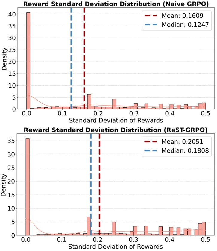
Figure 3: Paper Figure 1. (a) Reward variance becomes more informative during ReST-GRPO. (b) ReST-RL improves Qwen3-8B on code and provides transfer evidence on math and science without target-domain tuning. The paper is careful to note that reward standard deviation is only a proxy for the informativeness of group-relative updates; final attribution belongs to Table 3.

Training efficiency. Llama-3-8B is trained for 10k steps and evaluated every 1k steps to compare ReST-GRPO with DAPO and naive GRPO (Figure 3(a)). A general base is chosen because it leaves substantial room for coding improvement, which makes differences in optimization efficiency easier to observe than on a heavily code-specialized checkpoint. The three methods are comparable during the first 2k steps, after which ReST-GRPO's lead grows: at 10k steps its improvement is 12.3%, versus 7.8% for naive GRPO and 8.1% for DAPO.

More consequential is the end-to-end compute accounting of Table 4, which charges ReST-GRPO for its one-time offline sampling cost:

Method (Llama-3-8B, 10k steps)	Pre-sampling time (h)	Total training time (h)	Total GPU hours	Time to 6% gain	Time to 9% gain	Time to 12% gain
GRPO	0	260	2080	52 h	207 h	>260 h
ReST-GRPO	10	219	1752	51 h	71 h	199 h

Table 2: End-to-end training-time assessment (paper Table 4). Both methods run the same total number of steps and samples, and ReST-GRPO's pre-sampling time is always included.

These numbers are worth unpacking. ReST-GRPO spends 10 extra hours on offline sampling yet uses 328 fewer total GPU hours (1752 against 2080), and reaches a 9% improvement in 71 hours instead of 207. Appendix A.8 explains why: the main bottleneck of RL training is repeated online sampling and policy optimization, whereas offline pre-sampling is highly parallelizable and adds only limited latency; more importantly, the filtered and partially reassembled training data let the policy reach the same or higher performance in fewer effective optimization steps. The offline stage is amortized by fewer online hours, not added on top of them.

Figure 4: Paper Figure 3(a). Training-efficiency curves for ReST-GRPO, DAPO and GRPO on average benchmark score with Llama-3-8B, trained for 10k steps and evaluated every 1k steps.

Component Attribution and Matched Controls: The Hardest Experiments in the Paper

The authors are explicit that a rise in reward variance is an optimization statistic and cannot serve as evidence of final task performance, so diagnostics and downstream attribution are reported separately. Table 3(a) decomposes the components one at a time with matched optimizer, matched reward, $G=8$ and 2,000 updates, with applicable variants reusing the same offline trajectories:

Table 3(a) policy components	APPS-500	BCB	Table 3(b) matched policy-value pipelines	APPS-500	BCB
Naive GRPO	0.180	0.416	GRPO (policy only)	0.403	0.436
Filtering-only	0.193	0.429	GRPO + matched VM-MCTS	0.538	0.449
E2H-C curriculum baseline	0.189	0.418	ReST-GRPO (policy only)	0.565	0.476
Partial-only	0.190	0.425	ReST-GRPO + matched VM-MCTS	0.642	0.506
Uniform-prefix	0.187	0.418	Table 3(c), approximately matched latency: VM-BoN ($N=260$) 0.619 at about 41.5 s; VM-MCTS ($n=5,T=20$) 0.642 at 41.5 s
Full ReST-GRPO	0.207	0.440	VM-BoN latency is the calibration target, so per-prompt wall clock is identical

Table 3: The three controlled panels of paper Table 3. Panel (a) matches optimizer, reward, $G=8$ and 2,000 updates; panel (b) matches each value model to its generating policy; panel (c) fixes policy and value model while approximately matching latency.

Table 3(a) supports three readings. Filtering alone helps (0.180 to 0.193). Partial-state starts alone help (0.180 to 0.190). But only their combination is best (0.207/0.440). The E2H-C curriculum baseline reaches just 0.189/0.418: it changes which original prompts are sampled over time, whereas ReST-GRPO additionally changes where within a trajectory online RL resumes. Exponential prefix sampling also beats uniform sampling (0.207 against 0.187), because it favors earlier prefixes and therefore leaves a larger suffix action space.

Table 3(b) is the experiment that answers the methodological question posed earlier. Value-model initialization, architecture, the 1.1M targets, collection parameters, optimization steps, random seed and VM-MCTS configuration are all held fixed; the only variable is the policy that generated those trajectories. A GRPO-trained value model lifts its own policy from 0.403 to 0.538, showing that learning a state-localized value model benefits either policy; the matched ReST-GRPO pipeline reaches 0.642/0.506. So the first-stage policy-induced advantage does survive matched value learning and search, rather than merely producing a better policy-only checkpoint. Mechanism-level evidence is added in Appendix Table 6: under the same MCTS collection procedure used for value-model training, mean trajectory rewards for Base/GRPO/ReST-GRPO are 0.37/0.56/0.68 and medians are 0.01/0.60/0.78.

Table 3(c) handles a fairness issue that is easy to overlook: equal candidate counts do not imply equal latency. Holding the ReST-GRPO policy and the value model fixed and aligning mean wall-clock time to roughly 41.5 seconds per prompt, VM-MCTS obtains 0.642 while VM-BoN calibrated at $N=260$ obtains 0.619. Because policy, verifier and latency are all controlled, the remaining difference cleanly isolates whether the value model is used during tree allocation or only for final reranking.

Comparison With Decoding and Verification Methods

Table 2 compares ReST-RL against ORM+BoN, PRM+BoN, ORM-MCTS and VM-MCTS with the verification budget fixed at 100 candidates. The ORM is Skywork-Reward-Llama-3.1-8B-v0.2; the PRM is a Qwen2.5 process reward model trained with an improved Math-Shepherd method, using the minimum action-level reward of a single output as its verification score. Because the candidate budget is identical, what this table measures is sample efficiency.

Method (average over all benchmarks, verification on 100 samples)	Qwen3-8B	Qwen2.5-Coder-7B-Instruct	DS-Coder-6.7B-Instruct	OpenCI-DS-6.7B
Base	0.503	0.563	0.493	0.486
ORM	0.531	0.592	0.542	0.537
PRM	0.516	0.591	0.539	0.532
ORM-MCTS	0.538	0.588	0.547	0.535
VM-MCTS	0.615	0.652	0.576	0.569
ReST-RL	0.689	0.673	0.584	0.583

Table 4: Average results of ReST-RL and the reward-verification methods across all benchmarks (paper Table 2). ReST-RL is the global optimum obtained by combining with the best policy from Table 1.

VM-MCTS improves over the strongest listed baseline by 11.2%, 8.9%, 8.3% and 8.3% across the four bases. Its lead over ORM-MCTS is particularly telling: both use MCTS, and the only difference is whether the guidance signal is an ORM that scores completed outputs or a value model that estimates partial states. That gap therefore directly supports using a state-localized value estimate during decoding rather than only scoring finished outputs. It is also worth noting that the PRM scores below the ORM on Qwen3-8B (0.516 against 0.531), which runs against the common claim that PRMs verify more accurately than ORMs. The paper does not elaborate, but its value-target formulation happens to sidestep both problems that afflict PRMs here: dependence on step annotation, and a notion of "step correctness" that does not hold in the code domain.

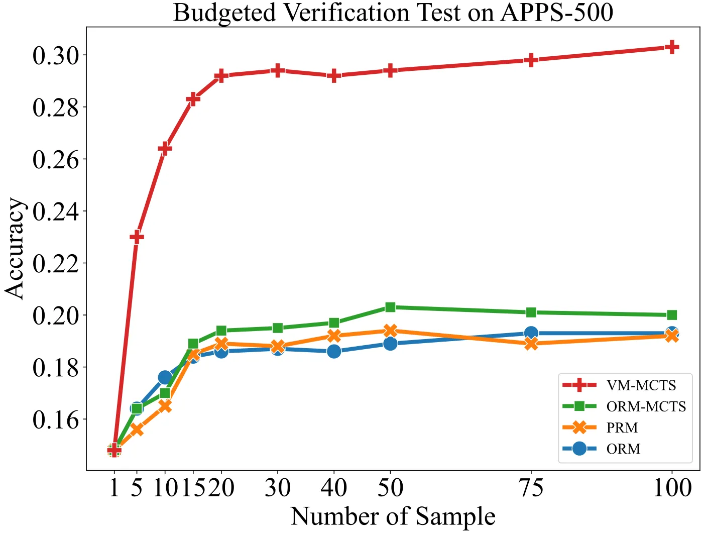
Figure 5: Paper Figure 3(b). Budgeted verification on APPS-500 with CodeQwen; sampling temperature is 0.7 for all methods. VM-MCTS stays ahead across the tested range, and Appendix Table 10 shows APPS-500 rising smoothly from the policy-only 0.565 to 0.652 as the branch factor $n$ grows, indicating a smooth compute-performance trade-off rather than dependence on one branch factor.

Latency and token cost. Appendix Table 18 gives the equal-sample view: on the base Qwen3-8B policy with 100 candidates each, ORM-BoN takes 16.0 s per prompt for 0.214 on APPS-500, VM-MCTS ($n=5,T=20$) takes 41.5 s for 0.415, $n=10,T=10$ takes 36.4 s for 0.355, and $n=20,T=5$ takes 28.6 s for 0.327. VM-MCTS is thus 1.8 to 2.6 times slower than ORM-BoN depending on tree shape, while nearly doubling accuracy. The paper's positioning is explicit: VM-MCTS is most appropriate where quality warrants additional latency, not in strict real-time settings. On token usage (Appendix Table 8), CodeQwen at $N=100$ spends 25,564 tokens for Best-of-N against 22,427 for VM-MCTS, so the search is not more token-hungry than plain sampling.

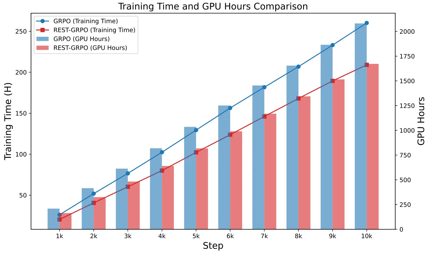
Figure 6: Paper Figure 4. Training time and the corresponding GPU-hour accounting for Llama-3-8B, comparing ReST-GRPO with naive GRPO, recorded every 1000 steps. Note that this figure does not include ReST-GRPO's pre-train sampling time; the full end-to-end comparison is Table 2 above.

Cross-Domain Transfer and Output Diversity

Table 5 asks whether a policy and a value model trained only on code trajectories remain useful out of domain and after policy updates. The paper's wording here is deliberately careful: coding remains the principal empirical domain, and this experiment tests transfer without target-domain tuning rather than claiming a universal reasoning value model.

Qwen3-8B configuration	APPS-500	BCB	MATH	Omni-MATH	GPQA-Diamond
Base (0th)	0.118	0.418	0.780	0.234	0.449
Base (0th) + VM (0th)	0.415	0.471	0.828	0.238	0.460
ReST-GRPO (2nd) + VM (0th)	0.630	0.496	0.862	0.246	0.480
ReST-RL (2nd, policy and VM matched)	0.642	0.506	0.872	0.256	0.490

Table 5: Preliminary cross-domain transfer results with Qwen3-8B (paper Table 5). The value model is trained only on code trajectories and receives no target-domain tuning. The third row deliberately pairs the initial value model with a policy that has already been updated twice, to assess robustness to policy shift.

Three conclusions follow. First, adding the code-trained value model to the base policy lifts MATH/Omni-MATH/GPQA-Diamond from 0.780/0.234/0.449 to 0.828/0.238/0.460, so there is genuine out-of-domain gain. Second, the initial value model remains useful after two rounds of policy updates (0.862/0.246/0.480), indicating robustness to moderate policy shift. This matters a great deal for deployment: since $V^{\pi}$ is policy-dependent in theory, the method would lose much of its value if every policy tweak forced a value-model retrain. Third, updating the value model to the final shifted policy yields the best 0.872/0.256/0.490, so matching still beats mismatching. The paper's reading is that the domain-agnostic objective $V^{\pi}(s)=\mathbb{E}_{\pi}[R\mid s]$ can transfer across task and policy shifts.

Does diversity collapse? This is the natural worry about any method that biases training toward high-reward trajectories: does it suppress exploration and collapse the output distribution? Appendix Table 19 answers no. Self-BLEU, computed by sampling 8 answers per prompt where a higher score means lower diversity, is 0.610 for Base, 0.620 for GRPO, 0.602 for ReST-DPO and 0.613 for ReST-GRPO. ReST-GRPO sits close to the base model and below GRPO. The paper's explanation is consistent with the design: ReST-GRPO does not deterministically replay a single trajectory but reshapes the training distribution by combining prompt-level filtering with partial-state sampling, so optimization is biased toward promising regions without eliminating variability in subsequent rollouts. Had the gains come mainly from collapse onto a narrow set of patterns, Self-BLEU would have risen sharply, and it did not.

Hyperparameter sensitivity. Appendix Table 9 varies $\sigma_0$, $\alpha$ and $r_0$ individually, training Qwen3-8B for 1k steps per setting; the performance range is relatively narrow and the default configuration is strongest overall. Practical guidance is offered as well: with rewards in $[0,1]$, $\sigma_0$ can start in a small range such as $(0,0.1)$ to avoid discarding informative prompts; in $p(j)\propto\alpha^{j-1}$ a lower $\alpha$ concentrates mass on shorter prefixes while $\alpha$ near one approaches a uniform distribution over prefix lengths, and 0.95 gives a mild early-prefix bias in this setting; stricter $r_0$ favors more reliable high-reward anchors; and $n$ and $T$ for VM-MCTS should be chosen against the available latency budget. The proxy analysis in Appendix Table 7 shows filtering raising mean reward standard deviation from 0.104 to 0.148, with high-reward trace selection and partial-state sampling pushing it further to 0.168, but the paper again stresses this characterizes the training signal only, with downstream attribution reported separately in Table 3.

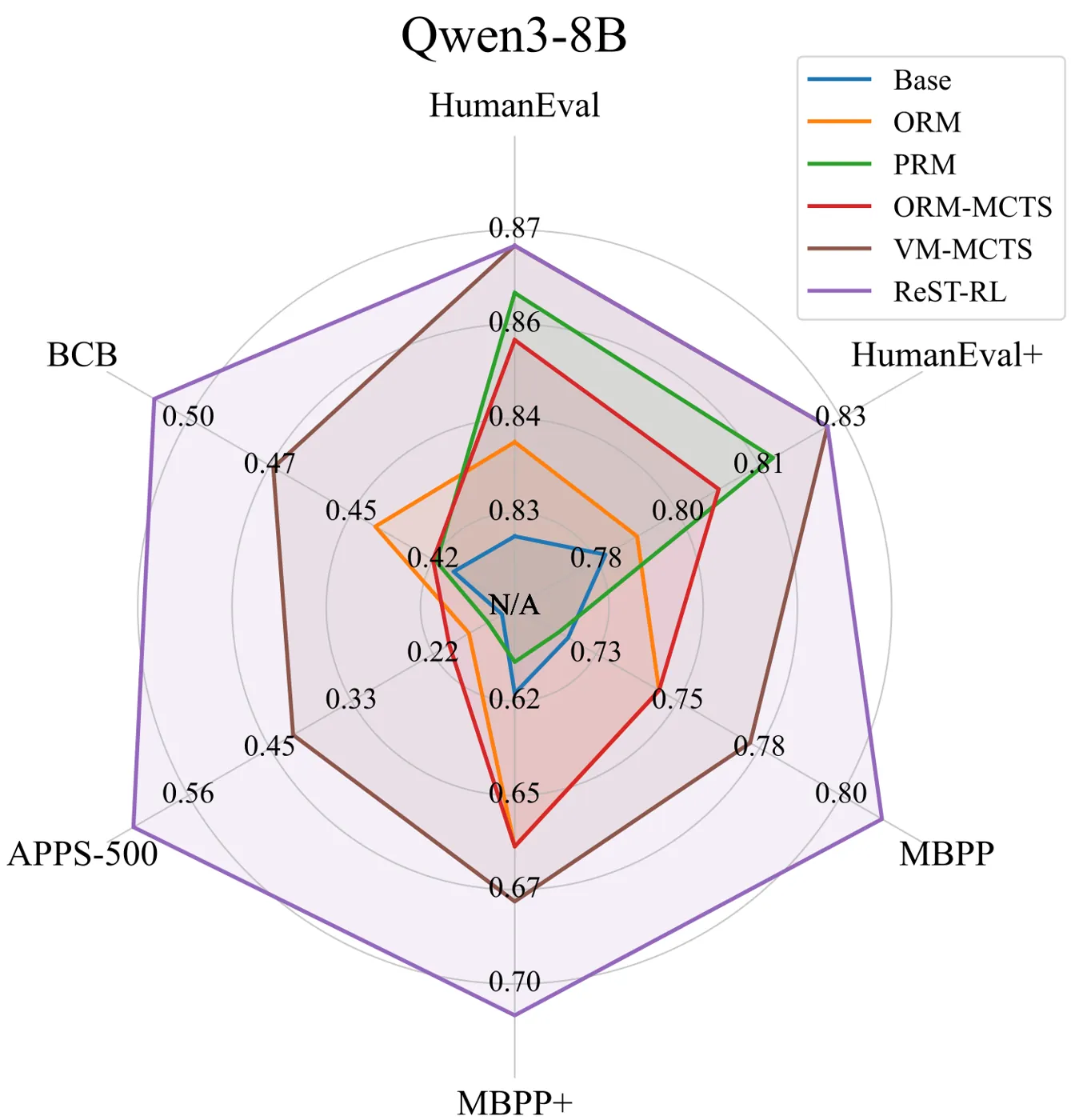
Figure 7: Paper Figure 5. Performance of different base LLM policies when using ReST-RL and the verification methods on all benchmarks. All verification is based on 100 samples with sampling temperature 0.7.

Limitations

Repeated multi-round policy-value coupling is not studied (stated by the authors). The paper reports only the two-stage pipeline: train the policy, freeze it, train the value model, decode. Iterating an updated policy against an updated value model over several rounds is not attempted. The third row of Table 5 is a shadow of this gap: the initial value model paired with a twice-updated policy still works, but that is evidence of robustness under mismatch, not evidence that iterative coupling would help. In principle the value model learns $V^{\pi}$, so every policy change moves the target; whether repeated coupling converges, and whether it is worth the cost, is left unanswered.

VM-MCTS has higher latency than BoN at equal candidate counts (stated by the authors). The authors say so plainly and note that the approximately latency-matched control is reported only on Qwen3-8B and APPS-500, so it does not cover every deployment regime. Combined with Appendix Table 18, VM-MCTS is 1.8 to 2.6 times slower than ORM-BoN under equal samples; Table 3(c) shows VM-MCTS still wins once latency is matched, but that is a single data point (0.642 against 0.619, a margin of 2.3 points). Latency-sensitive production code generation cannot adopt this recipe as-is.

The controlled runs use one training seed and one base model (stated by the authors). Both the component controls of Table 3(a) and the matched value-model runs of Table 3(b) are single-seed, single-base. The authors point out that the main ReST-GRPO result is supported by four independent runs across multiple model families, but the two most persuasive controlled experiments in the paper have the smallest sample size. The 10-point gap between 0.538 and 0.642 is very likely real; the differences among the Table 3(a) variants at 0.187/0.189/0.190/0.193, all within 0.6 points, are essentially undecidable under a single seed.

The math and science experiments do not establish a universal verifier (stated by the authors). The transfer results use Qwen3-8B alone and demonstrate transfer without target-domain tuning, not the existence of a universal reasoning value model. In absolute terms the out-of-domain gains are small: Omni-MATH moves from 0.234 to 0.256 (+2.2 points) and GPQA-Diamond from 0.449 to 0.490 (+4.1 points), which is not in the same league as the +52.4 points on APPS-500 (0.118 to 0.642) in the code domain.

Value-target noise and reward shaping are two openings that are not cleanly quantified (this reviewer's judgment). The paper itself says the value target introduces some extra noise yet performs better under MCTS decoding, and offers the variance argument of Appendix A.12. That argument rests on a fairly strong set of assumptions: that $V_{\phi}$ and $R_{\lambda}$ are both unbiased, have equal variance, and have noise independent of the state. Whether a model regressed with MSE on 1.1M self-collected targets is actually unbiased is never measured. Separately, the reward shaping of Equation 7 (required substring plus redundant-character penalty) is used by ReST-GRPO and naive GRPO alike, so the comparison is fair, but it does mean the reported absolute scores depend on that layer of engineered reward design. Moving to a new domain requires redesigning $\omega_1$, $\omega_2$ and the definition of the required substring.

Line-level action granularity is not ablated outside the code domain (this reviewer's judgment). Appendix A.8 supports the choice by citing recent work such as LSR-MCTS, DISC and ReSCALE, noting that newline-delimited units often correspond to semantically coherent reasoning segments and that PRM800K-style steps are commonly organized line by line. But these are cited supports, not the paper's own ablation: no domain is used to compare line-level against token-level actions, or line-level against reasoning-step-level actions. The authors report the motivation and the engineering convenience of the choice, and they themselves list adaptive or task-specific action abstractions as an important direction.

Conclusion and Outlook

The contribution of ReST-RL can be read as two acts of reconnecting a signal. The first reconnects state-level information on the training side: GRPO removed reward learning from the RL loop entirely in order to stay lightweight, and this paper brings state-level guidance back without introducing a value network into training, by letting online RL resume from the middle of a successful trajectory instead of restarting from the original prompt every time. The second reconnects fine-grained information on the inference side: not an ORM that scores completed outputs, not a PRM that needs step annotation, but a value model predicting expected terminal reward, trained on self-collected MCTS targets, paired with a static policy, and used for both search allocation and final selection.

The most valuable part of this work may not be the final 0.689 but its attitude toward what counts as proof. The paper demotes reward standard deviation to a proxy, hands component attribution to the downstream results of Table 3(a), hands the two-stage dependency claim to the matched controls of Table 3(b), and hands the "equal candidates does not mean equal latency" trap to the wall-clock-aligned panel of Table 3(c). It even records honestly that the historical construction seed of the APPS-500 subset is unavailable and that the math and science results are preliminary transfer evidence. This discipline in reporting diagnostics separately from task performance is not common in a methods paper.

Two engineering lessons transfer directly. First, end-to-end compute accounting must include the offline stage: ReST-GRPO spends 10 extra hours pre-sampling yet saves 328 GPU hours, because highly parallelizable offline sampling buys fewer effective online optimization steps. That trade-off holds in many pipelines that build data offline and then train online. Second, value models are more reusable than theory suggests: the initial value model paired with a twice-updated policy still delivers (third row of Table 5), so in practice a value model need not be retrained after every policy tweak, which sharply lowers the maintenance cost of this approach in a continuously iterated system.

The open questions are equally clear: whether multi-round policy-value coupling converges and pays for itself; whether the unbiasedness of $V_{\phi}$ can be measured rather than assumed; whether line-level action granularity needs adaptive abstraction outside code; and whether the 2.3-point advantage in Table 3(c) survives a strict latency budget. The paper's own positioning is restrained. It does not claim to have built a universal reasoning value model, only to have reconnected policy optimization and value-guided reasoning without paying the full price of online actor-critic learning.

Golden Quotes

"Selected prefixes are not treated as imitation targets: they become additional online-GRPO contexts from which the policy samples and optimizes fresh suffixes."

"Connecting these roles is useful only if the first-stage policy improvement survives a matched value-learning pipeline rather than merely producing a better policy-only checkpoint."

"Our framework reintroduces that missing signal in a lightweight manner. It is an attempt to reconnect policy optimization and value-guided reasoning without returning to the full cost of online actor-critic learning."