HyperDCM: Dynamic Cluster Memory Replay in Hyperbolic Space for Continual Robotic Navigation Across Scenes

Paper: HyperDCM: Dynamic Cluster Memory Replay in Hyperbolic Space for Continual Robotic Navigation Across Scenes
Authors: Zhengfei Lu, Jian Yang, Muyu Wang, Shaowen Chen, Jinpeng Mi, Ke Li, Xiong You, Qi Wu, Xuan Tang, Xian Wei
arXiv: 2607.16267
Code status: No public code is provided in the paper, and GitHub search did not reveal a reliable official implementation.

Summary: HyperDCM converts RGB observations into scene graphs, maps them to Poincare hyperbolic space, and maintains replay samples with structure-sensitive dynamic clustering. The result is a diffusion navigation policy that retains prior scenes while adapting to new ones.

Background and Motivation

Visual navigation is often presented as a perception problem, but its difficult part is behavioral. A robot does not merely need to recognize a hallway, table, curb, or doorway; it must produce a future trajectory that respects goal constraints, obstacles, and the temporal structure of locomotion. In deployed environments, the problem becomes worse because the mapping from observation to action is not fixed. Furniture moves, pedestrians appear, doorways close, lighting changes, and a policy trained in one building may be asked to operate in another.

Diffusion policies have become attractive for this setting because they model action generation as denoising rather than as direct regression. A regression model tends to average plausible futures. If a robot can pass to the left or right of a table, an averaged action may approach the table from an awkward angle or fail to satisfy either mode. A diffusion policy can instead represent multi-modal action distributions and refine noisy action sequences into feasible waypoint trajectories. This is particularly useful for goal-conditioned navigation, where one context may require exploration and another may require direct goal pursuit.

The authors frame the remaining issue as memory. Most diffusion navigation policies are trained on static, closed datasets. They are not designed to learn scene one, then scene two, then scene three without damaging earlier behavior. When the model updates its parameters for a new scene, the denoising patterns associated with old scenes can disappear. This is catastrophic forgetting, and it is especially problematic for diffusion policies because their generation process often relies on pixel-level or vectorized features that do not explicitly encode how objects and places are related.

A conventional replay buffer offers one answer: keep some old samples and mix them with current data. This helps, but uniform replay treats every retained trajectory as equally valuable. Navigation experiences are not flat. A room contains a table, a table supports objects, a doorway connects to a corridor, and a corridor connects rooms. These relations form a hierarchy. If the buffer is selected by pixel similarity or random sampling, it may keep many near-duplicate scenes while losing structurally distinct experiences.

HyperDCM starts from a different assumption: a good memory should know what makes experiences structurally different. The paper uses scene graphs to represent observations as subject-predicate-object triples, then uses hyperbolic geometry to preserve hierarchical relations. The goal is not to replace the diffusion policy but to surround it with a memory mechanism that selects and organizes replay samples more intelligently.

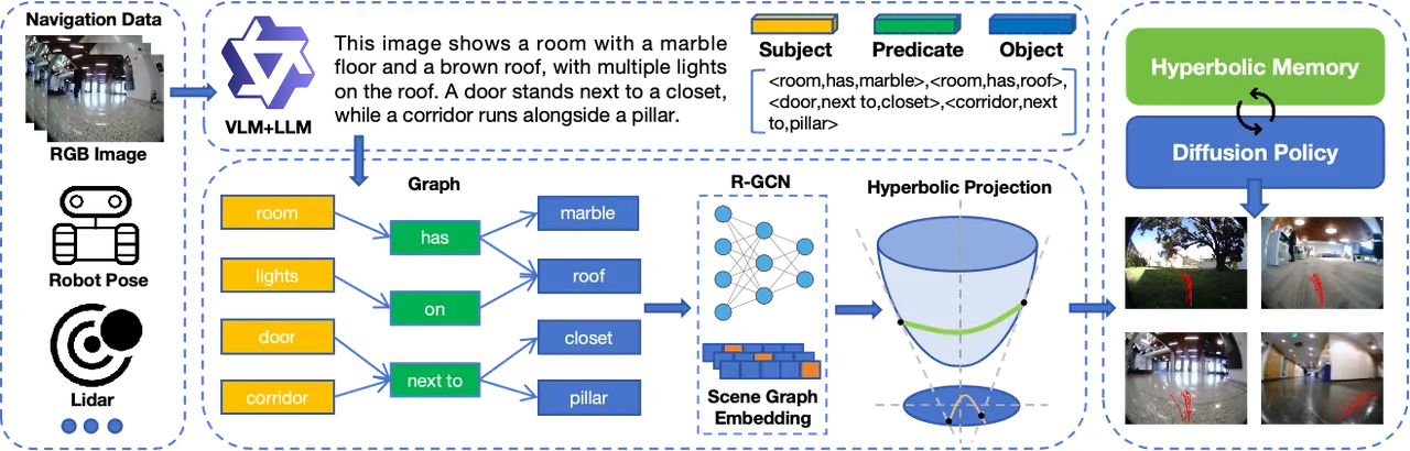
Figure 1: HyperDCM overview. RGB trajectories are processed by vision-language models into semantic descriptions, parsed into triples and scene graphs, encoded by an R-GCN, and projected into hyperbolic space for dynamic replay.

Preliminaries: Policy Learning and Memory Geometry

Diffusion-based navigation begins with a noisy action sequence and repeatedly denoises it into a feasible trajectory. The model is conditioned on the current observation and navigation goal. This formulation has two useful properties. First, it can represent several valid routes rather than collapsing them into a single average path. Second, it can generate multiple future waypoints, giving the policy temporal foresight instead of making every step an isolated decision.

Continual learning research offers three broad families of solutions. Regularization methods constrain important parameters from moving too far. Replay methods store representative past samples and interleave them with new data. Parameter isolation allocates separate capacity to different tasks. In robot navigation, replay is especially practical because it does not require changing the policy backbone or maintaining a large set of task-specific modules. The hard part is therefore not whether to replay, but which samples to retain when memory is bounded.

A scene graph provides the semantic identity of an experience. Instead of describing an image as a bag of detections, it records entities and their relations. R-GCN is a natural encoder for this structure because different relation types can use different learned transformations. The resulting embedding captures both object semantics and topology. HyperDCM treats this embedding as a stable signature of a navigation experience.

Hyperbolic space supplies the geometric prior. In the Poincare disk, geodesic distances expand rapidly near the boundary, giving more representational room to hierarchical branching. This is valuable for scene graphs, which often resemble trees: rooms contain tables, tables support objects, and doorways connect areas. The paper shows UMAP visualizations in which Poincare embeddings separate scene-level memory samples more cleanly than Euclidean embeddings.

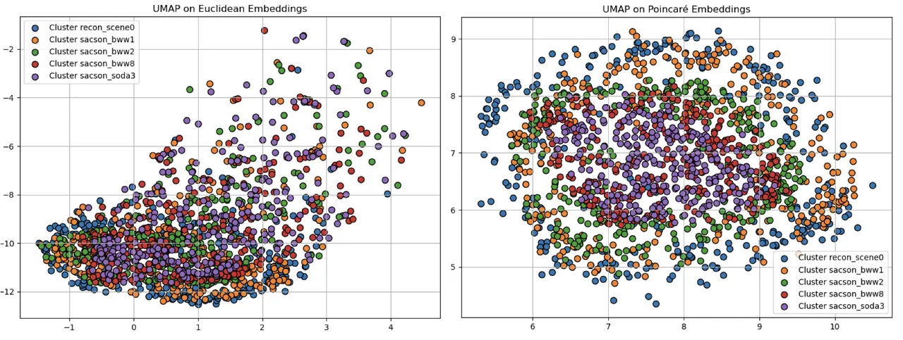
Figure 2: UMAP visualization of Euclidean and Poincare embeddings. The hyperbolic representation shows stronger separation and local clustering, suggesting better preservation of structural relations.

Method

HyperDCM has three stages. First, raw RGB observations are converted into structured scene graphs. Second, graph embeddings are projected into hyperbolic space. Third, new samples are assigned to dynamic clusters, cluster centers are updated with hyperbolic geometry, and representative samples are replayed during diffusion-policy training. Figure 3 shows the overall memory-management loop.

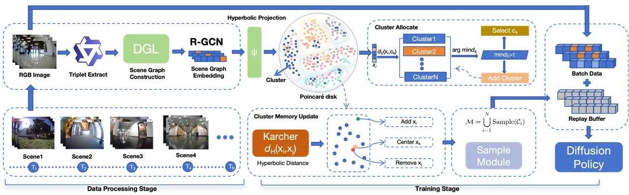
Figure 3: Dynamic cluster memory management. Euclidean distance is used for fast assignment, while hyperbolic distance and Karcher centers guide updates and replacement.

Structured Scene Graph Representation

The pipeline starts from RGB observations collected during robot trajectories. Qwen-VL converts an image into a textual description, and Qwen3-7B parses that description into semantic triples $(s,r,o)$, where $s$ is a subject, $r$ is a relation, and $o$ is an object. This step is performed offline and avoids handcrafted relation rules. It also gives the memory mechanism a language-level interface to scene content.

The triples form a scene graph, and an R-GCN performs relation-aware message passing. The paper writes the node update as:

$$h_i^{(l+1)}=\sigma\left(\sum_{r\in\mathcal{R}}\sum_{j\in\mathcal{N}_{r}(i)}\frac{1}{c_{i,r}}W_r^{(l)}h_j^{(l)}+W_0^{(l)}h_i^{(l)}\right)$$

Here $\mathcal{R}$ is the set of relation types, $\mathcal{N}_r(i)$ is the neighbor set of node $i$ under relation $r$, and $c_{i,r}$ is a normalization constant. $W_r^{(l)}$ transforms messages associated with relation $r$, while $W_0^{(l)}$ transforms the node's own state. The resulting scene embedding $z_i\in\mathbb{R}^{128}$ is passed to hyperbolic projection and memory clustering.

An important implementation choice is that the R-GCN is used only for offline embedding generation. Its weights are fixed after preprocessing. This means the graph encoder is not continuously moved by gradients from new scenes. Its role is to provide a stable coordinate system for memory rather than to act as another trainable policy component that itself forgets.

Poincare Mapping

Euclidean embeddings can compress hierarchical structures into a metric space that is not naturally suited to them. Two scenes may share similar object sets but differ in how those objects are organized. A room containing a table differs from a table supporting objects, and a corridor that connects several rooms has a different structural role from an isolated doorway. Hyperbolic geometry gives these differences more room by expanding distance near the boundary of the disk.

HyperDCM projects the Euclidean scene embedding $z_i$ into the Poincare disk with a fixed curvature $c$:

$$\phi(z_i)=\frac{z_i}{\sqrt{c}(\|z_i\|+\epsilon)}\cdot\tanh(\sqrt{c}\|z_i\|)$$

The curvature parameter $c$ controls the geometry, and $\epsilon$ stabilizes computation. The authors state that the same curvature is used across all scenes and is held fixed during final evaluation. This is important for memory consistency: samples collected at different stages of continual learning are comparable within one metric system.

The Poincare distance between two points is:

$$d_{\mathbb{H}}(\mathbf{u},\mathbf{v})=\operatorname{arcosh}\left(1+\frac{2\|\mathbf{u}-\mathbf{v}\|^2}{(1-\|\mathbf{u}\|^2)(1-\|\mathbf{v}\|^2)}\right)$$

As $\mathbf{u}$ or $\mathbf{v}$ approaches the boundary, the denominator shrinks and the geodesic distance grows. Thus a structurally rich scene graph is not simply treated as an outlier because its norm is large; it occupies a region of the disk that matches its hierarchical complexity.

Dynamic Clustering and Scheduling

The memory contains $C$ clusters, each with capacity $M$. For a new embedding $\phi(z_i)$, the system first computes Euclidean distances to all cluster centers $\{c_k\}_{k=1}^{C}$ and selects the nearest center:

$$\min_{k\in\{1,...,C\}}d_E(\phi(z_i),c_k)$$

If the minimum distance exceeds threshold $\tau$ and the cluster limit has not been reached, a new cluster is created. Otherwise, the sample is assigned to the nearest existing cluster. Once the maximum number of clusters is reached, new samples are assigned to the nearest cluster so that memory growth remains bounded.

Within a cluster, the mechanism uses the Karcher mean instead of a Euclidean mean. The Karcher mean generalizes the mean to a Riemannian manifold. For the hyperbolic memory set, it is defined as:

$$\mu=\arg\min_{y\in\mathcal{M}}\sum_{i=1}^{N}d_{\mathbb{H}}^2(y,x_i)$$

For a particular cluster $C_k$, the center $\bar{x}_k$ satisfies:

$$\bar{x}_k=\arg\min_{x\in\mathbb{D}^{n}}\sum_{x_j\in C_k}d_{\mathbb{H}}^2(x,x_j)$$

In practice, the paper updates the affected center with a small fixed number of Riemannian gradient steps. Because both the number of clusters and per-cluster capacity are bounded, this update has bounded overhead. It also avoids a common failure mode of Euclidean averaging, where the average of valid points on a curved manifold may not itself be a meaningful point on that manifold.

The replacement rule is the most distinctive part of the memory update. Let $\tilde{x}_i$ be a new sample. Its hyperbolic distance to the cluster center is $d_{\mathbb{H}}(\tilde{x}_i,\bar{x}_k)$. The current cluster member closest to the center is $x_j$. If $d_{\mathbb{H}}(\tilde{x}_i,\bar{x}_k)>d_{\mathbb{H}}(x_j,\bar{x}_k)$, HyperDCM replaces $x_j$ with $\tilde{x}_i$.

The intuition is that samples close to a cluster center are already structurally represented, while samples farther from the center, but still assigned to that cluster, may capture unusual branches, boundary conditions, or rare relations. Keeping those samples prevents the replay set from collapsing into many near-duplicates. A memory that always preserves central examples becomes conservative; a memory that preserves controlled distance from centers retains diversity.

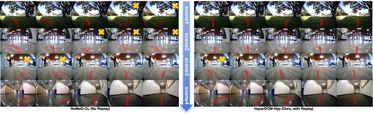
Figure 4: Predicted waypoint trajectories in four representative scenes. The continual NoMaD baseline drifts on earlier scenes, while HyperDCM-Hyp keeps smoother and better goal-aligned predictions.

Replay Sampling

During training, the replay batch is sampled uniformly from the union of all clusters:

$$\mathcal{B}=\text{Sample}\left(\cup_{k=1}^{C}\text{Cluster}_{k},\text{size}=n\right)$$

These samples are combined with the current scene data to fine-tune the diffusion policy. Because sampling is organized around clusters rather than raw frequency, each structural group can influence training. Rare but important topological relations are not drowned out by repetitive visual content.

The memory pipeline is modular. It does not modify the diffusion-policy backbone. It observes, encodes, clusters, replaces, and replays samples around the policy. That modularity makes HyperDCM easier to attach to NoMaD-style navigation models and allows a fair comparison with EWC, SI, LwF, and TinyER under the same continual-learning protocol.

Why the Design Fits Diffusion Navigation

Diffusion navigation policies are sensitive to the distribution of trajectories used during denoising. They are not merely fitting a final end point; they are learning a conditional vector field over an action sequence. If the training distribution becomes dominated by a newly introduced scene, the model's denoising process can lose support for previously learned maneuver families. Replay therefore needs to restore not just samples from old scenes, but the diversity of relational contexts under which those samples were valid.

This is where scene graphs have a practical role. Pixel-level features can encode that a table is present, but they may not make explicit whether the table is central to the route, adjacent to the goal, or connected to a doorway that constrains movement. A subject-predicate-object representation turns those distinctions into graph topology. The R-GCN embedding can then place a dining-room experience with a similar object set but a different route topology closer to other navigationally similar experiences.

Hyperbolic projection adds a second, subtler benefit. Scene graphs are rarely complete Euclidean grids. They are sparse, branching, and often hierarchical. In a Euclidean memory, the distance between a room and its contained objects can be distorted by dimensional limitations. In a Poincare disk, the geometry itself expands room for deep or branching relations. This does not guarantee better navigation, but it gives the memory mechanism a better prior for distinguishing experiences that look visually similar while occupying different structural roles.

The combination also explains why HyperDCM does not simply become a retrieval system. The policy still learns from current observations and actions. Memory only controls which past experiences are reintroduced into optimization. This keeps the computational burden away from online inference. Scene-graph extraction is offline, clustering is incremental, and replay sampling is a standard training-time operation.

The separation of metric duties is also pragmatic. Euclidean nearest-center assignment is cheap and sufficient to decide where a new embedding should live. Hyperbolic distance is more expensive but is reserved for center updates and replacement decisions, where geometric fidelity matters most. This engineering choice matters for a robot system: the memory must scale across scenes without making every new observation trigger a costly manifold optimization.

Reading the Evidence

The continual-learning protocol is stricter than a simple train-test split because the model's state changes after every scene. The notation $1\sim A$ through $1\sim E$ therefore measures a moving system, not five independent models. A method can look strong at an early checkpoint and still be weak if its later updates erase earlier competence. This is why the Drop metric is useful: it summarizes retention across the whole sequence rather than rewarding a single high point.

The baseline behavior is informative. NoMaD-CL starts at 70.0 on the first-scene evaluation, even higher than Joint NoMaD's 66.5 at that point, but falls to 26.7 after later scenes. The early advantage does not indicate better lifelong learning; it shows that a policy trained only on one scene can overfit that scene and then lose it. Regularization methods reduce forgetting, but they do not reintroduce the data diversity that the diffusion denoiser needs.

TinyER demonstrates the value of replay, yet its improvement is limited. Uniform random replay keeps old examples, but it does not decide whether the buffer contains redundant samples. The result is a Drop of 36.9, only a few points better than LwF. This supports the paper's claim that the central issue is not replay itself but the organization of replay.

HyperDCM-VisFeat separates that issue. It still uses cluster-based memory and hyperbolic projection, but it removes the scene graph and uses visual features instead. Its Drop improves to 35.2, showing that structured clustering alone helps. The fact that it still underperforms the full model indicates that visual features alone do not capture the relational identity of navigation experiences.

HyperDCM-Euc keeps the structural clustering idea but replaces hyperbolic distance with Euclidean L2 distance. Its Drop improves slightly to 34.8. The small difference from VisFeat suggests that both components contribute, while the larger gap from HyperDCM-Hyp suggests that hyperbolic geometry is not merely a cosmetic transformation. It changes how centers and representative samples are chosen.

The strongest signal appears in the intermediate checkpoints. HyperDCM-Hyp reaches 55.2 at $1\sim C$ and 45.2 at $1\sim D$, while other continual methods stay between roughly 31 and 41. That means the method is not only preserving a small advantage until the last scene; it maintains a broader behavioral repertoire throughout training. This matters in deployment because a robot rarely knows in advance whether the next scene will be the last.

The Habitat online study then moves beyond trajectory prediction. SPL penalizes inefficient paths, so an improvement from 38.5 to 48.3 cannot be explained by memorizing a longer wandering route. Collision frequency falls from 0.37 to 0.17, which suggests that remembered structure helps the policy avoid unsafe behavior rather than merely reaching a threshold more often. Joint NoMaD still performs better, but it assumes access to all accumulated data.

The qualitative figure adds a necessary check. Numerical success rate can miss subtle trajectory degradation: a policy may reach the goal while oscillating, drifting near obstacles, or producing implausible waypoints. Figure 4 shows that the NoMaD baseline drifts in earlier scenes, whereas HyperDCM-Hyp preserves smoother and better goal-aligned paths. This aligns with the quantitative retention result.

Experiments

The authors construct five scene splits from the indoor SACSoN dataset and the outdoor Recon dataset. For each scene, 60 percent of trajectories are used for training and 40 percent for testing. Each trajectory contains robot-view images, pose information, and goal-conditioned annotations. The diffusion policy uses a NoMaD-style baseline and is trained on an NVIDIA RTX 4090. Each scene is trained for 20 epochs, and a checkpoint is saved after every stage to measure retention on earlier scenes.

The primary metric is success rate:

$$\text{SR}=\frac{1}{N}\sum_{i=1}^{N}\mathbf{1}\left[d(s_i,g_i)\leq\delta\right]$$

where $s_i$ is the final state of trajectory $i$, $g_i$ is the goal, and $\delta$ is the success threshold. The notation $1\sim X$ means that the model has been trained sequentially from Scene 1 through Scene X. The paper also defines Drop as $\text{SR}_{1\sim A}-\text{SR}_{1\sim E}$; larger Drop values indicate more forgetting.

The main trajectory-prediction results show a severe baseline failure. Without replay, NoMaD-CL drops from 70.0 success at $1\sim A$ to 26.7 at $1\sim E$, for a Drop of 43.3. Regularization methods help only moderately: EWC reaches 27.3 with Drop 40.1, SI reaches 27.6 with Drop 38.6, and LwF reaches 29.1 with Drop 37.4. TinyER reaches 28.6 with Drop 36.9. HyperDCM-VisFeat, which retains cluster replay but removes scene graphs, lowers Drop to 35.2. HyperDCM-Euc lowers it to 34.8. Full HyperDCM-Hyp reaches 41.5 with Drop 28.5.

Method	1~A	1~B	1~C	1~D	1~E	Drop ↓
Joint NoMaD	66.5	62.7	58.1	60.5	60.2	6.3
NoMaD-CL (No Replay)	70.0	40.6	34.4	25.2	26.7	43.3
NoMaD-CL + EWC	67.4	42.3	35.7	30.2	27.3	40.1
NoMaD-CL + SI	66.2	44.7	36.3	29.4	27.6	38.6
NoMaD-CL + LwF	66.5	46.1	38.5	33.9	29.1	37.4
NoMaD-CL + TinyER	65.5	45.5	37.6	31.5	28.6	36.9
HyperDCM-VisFeat	65.7	48.6	40.7	37.5	30.5	35.2
HyperDCM-Euc (L2)	66.7	48.2	41.1	36.0	31.9	34.8
HyperDCM-Hyp (Poincare)	70.0	50.8	55.2	45.2	41.5	28.5

The progression matters as much as the final number. Replay gives stability. Adding structure improves sample diversity. Hyperbolic geometry then improves long-term retention beyond Euclidean organization. The 55.2 and 45.2 values at $1\sim C$ and $1\sim D$ are especially important because they show that HyperDCM is not merely sacrificing old scenes slowly; it maintains stronger transferable representations throughout the sequence.

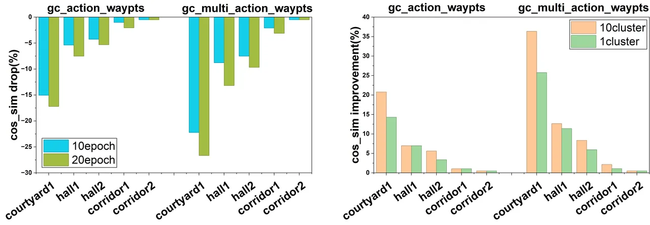
Figure 5: Trajectory-level forgetting analysis. Without replay, longer training amplifies cosine-similarity drop; with fixed memory size, clustered memory outperforms a single buffer.

The Habitat experiments provide an online navigation test on five MatterPort3D scenes. They report success rate, SPL, and collision frequency. NoMaD-CL without replay achieves 39.2 SR, 38.5 SPL, and 0.37 collisions per meter. TinyER reaches 41.7 SR. HyperDCM-Hyp reaches 56.0 SR, 48.3 SPL, and 0.17 collisions. Joint NoMaD remains the upper bound at 63.1 SR, 52.7 SPL, and 0.13 collisions.

Method	SR ↑	SPL ↑	Collision ↓
Joint NoMaD	63.1	52.7	0.13
NoMaD-CL (No Replay)	39.2	38.5	0.37
NoMaD-CL + TinyER	41.7	40.2	0.29
HyperDCM-VisFeat	45.0	42.0	0.24
HyperDCM-Euc (L2)	49.8	46.0	0.22
HyperDCM-Hyp (Poincare)	56.0	48.3	0.17

The ablation isolates the two contributions. HyperDCM-VisFeat removes the scene-graph encoder and directly embeds EfficientNet visual features into hyperbolic space. HyperDCM-Euc retains centroid-based replay but replaces hyperbolic distance with Euclidean L2 distance. Both degrade performance. This supports the paper's claim that hierarchical scene encoding and negative-curvature geometry are complementary rather than redundant.

Training efficiency is also favorable. Joint retraining visits all accumulated data at each new stage, so its GPU-hours grow approximately linearly with the number of scenes. HyperDCM keeps per-stage training cost nearly constant. Scene-graph extraction is offline preprocessing performed once per scene, and the reported GPU-hours count only diffusion-policy optimization. Joint retraining still achieves stronger adaptation to the newest scene, but HyperDCM offers a much lower-cost operating point.

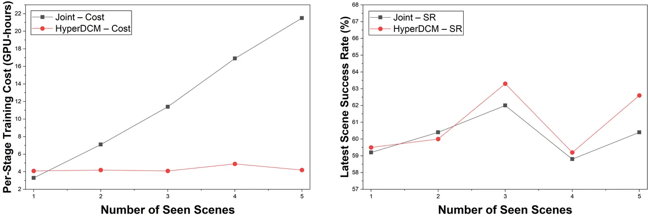
Figure 6: Joint retraining versus HyperDCM. The left plot shows per-stage GPU-hours; the right plot shows success rate on the latest scene.

Limitations

The first limitation is dependence on vision-language extraction. Qwen-VL and Qwen3-7B convert images into textual descriptions and triples, but the paper does not deeply quantify how hallucinated entities, missed relations, or wrong edges propagate into memory clusters. Long-tail objects, ambiguous occlusions, and linguistic uncertainty could place a sample in a structurally wrong region.

The second limitation is parameter rigidity. The clustering threshold $\tau$, number of clusters $C$, per-cluster capacity $M$, and curvature $c$ are fixed during evaluation. Fixed values make the study controlled, but real deployment may alternate between environments that need few broad clusters and environments with many fine-grained layouts. The authors explicitly identify adaptive memory allocation as future work.

The third limitation is the replacement heuristic. HyperDCM assumes that a sample farther from the Karcher center is structurally richer. This is plausible for hierarchical scene graphs, but distance can also increase because of noisy embeddings, anomalous detections, or incorrect relations. The paper does not report a replacement error rate or a sensitivity study for bad samples.

Fourth, the online simulation evaluation uses five MatterPort3D scenes. SACSoN and Recon add indoor and outdoor trajectory diversity, but long-duration deployment would introduce more dynamic agents, changing doors, lighting shifts, and sensor noise. The authors also point to model-generated replay samples as future work, which indicates that the current system still depends primarily on retained real samples.

Engineering Interpretation

For a robotics team, HyperDCM is best read as a memory-policy integration pattern rather than a monolithic architecture. The diffusion policy can remain unchanged, while the memory layer handles observation indexing and sample selection. This is valuable because navigation backbones evolve quickly; a memory design that is decoupled from the action head is easier to carry across model versions.

The offline nature of scene-graph extraction is both a strength and a boundary. It keeps expensive vision-language inference out of the control loop, which is important for real-time navigation. It also means the memory is only as fresh as the latest preprocessing pass. A rapidly changing environment may require re-extraction or incremental updates, and the paper does not yet define that online lifecycle.

The bounded cluster design is similarly practical. A lifelong robot cannot allow the number of clusters or per-cluster samples to grow without limit. HyperDCM addresses this by creating a new cluster only when the distance threshold and cluster cap permit, and by forcing assignment to the nearest cluster once the cap is reached. That gives deployment a predictable memory footprint.

The Karcher-center update is the part most likely to require implementation care. A naive Euclidean average of Poincare points can fall into an unrepresentative location, so the paper uses Riemannian gradient steps. A practical system would need to bound the number of update iterations, monitor convergence, and ensure that centers remain numerically stable near the disk boundary.

Replacement is also a policy decision, not just a mathematical one. Replacing the member closest to the center preserves distant examples, but it can still discard information if the closest member is the only example of a small submode. A future variant could protect rare labels, goal types, or failure cases before applying the distance rule.

The replay sampler is deceptively simple. Uniform sampling across clusters encourages structural coverage, but it does not weight clusters by task relevance, recency, or expected deployment distribution. In one building, a rare basement topology may matter; in another, it may be irrelevant. Adaptive allocation could improve this without changing the rest of the pipeline.

Finally, the method's usefulness depends on evaluation cost. Continual navigation benchmarks are expensive because every stage requires checkpoints and multiple evaluations. The paper's shared protocol across baselines is therefore important. It aligns scene order, optimizer, batch size, learning-rate schedule, epochs, replay capacity, and replay ratio, making the comparison more meaningful than a collection of disconnected continual-learning results.

Conclusion

HyperDCM advances continual robot navigation by changing what the memory preserves. Instead of asking only whether to replay, it asks how replay samples should be structured and compared. RGB observations become semantic triples; triples become scene graphs; R-GCN produces relational embeddings; Poincare mapping preserves hierarchy; dynamic clusters organize experience; and structure-sensitive replacement maintains diversity.

The experimental evidence is consistent. Without replay, five-scene success falls from 70.0 to 26.7. HyperDCM-Hyp recovers the final success rate to 41.5 and reduces Drop from 43.3 to 28.5. In Habitat online navigation, success rises from 39.2 to 56.0 and collision frequency falls from 0.37 to 0.17. Ablations support both the scene-graph representation and the hyperbolic geometry.

For robotics practitioners, the broader lesson is that memory is not just a bag of past experiences. It is a structured asset whose organization determines what future training can recover. Adaptive cluster allocation, generated replay samples, and online correction of erroneous relations are natural next steps. The paper's conclusion also suggests that structural world modeling combined with hyperbolic geometry may matter beyond navigation, especially for continual robot learning tasks where experience has hierarchy.

flowchart TD
  A[RGB trajectories] --> B[VLM description]
  B --> C[semantic triples]
  C --> D[scene graph]
  D --> E[R-GCN embedding]
  E --> F[Poincare mapping]
  F --> G{nearest cluster}
  G -- distance greater than threshold --> H[create cluster]
  G -- distance within threshold --> I[assign cluster]
  I --> J[Karcher center update]
  J --> K[structure sensitive replacement]
  H --> L[uniform cross cluster replay]
  K --> L
  L --> M[current scene batch]
  M --> N[finetune diffusion policy]
  N --> O[continual navigation]

Golden Lines

"Continual navigation is not only about learning a new scene well; it is about not losing the structure of old scenes while learning it."

"A memory that stores by similarity remembers pictures. A memory that stores by structure remembers how the environment is organized."