PAC-DP: PAC-Bayesian Diffusion Policy Learning

1. Overview: PAC-Bayesian Diffusion Policy Learning

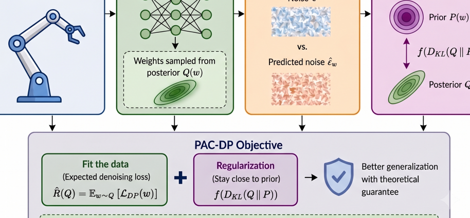
PAC-DP, proposed by Mohammad Hasan Yeganegi, Dian Yu, Andrea Del Prete, Majid Khadiv, and Matteo Saveriano in July 2026, models the diffusion policy as a Bayesian neural network and derives a novel training objective from PAC-Bayesian learning theory that augments the standard denoising loss with a KL-divergence regularizer between posterior and prior parameter distributions. While diffusion policies excel at complex manipulation tasks, minimizing the empirical denoising objective alone does not guarantee generalization in low-data regimes: the optimal score function can produce samples closely tied to training data, and diffusion models can memorize training samples when trained on limited datasets. PAC-DP provides a principled regularization mechanism grounded in statistical learning theory. Experiments demonstrate improved denoising accuracy, lower variational negative log-likelihood, and higher downstream robot task success rates compared to standard DP, with the largest improvements observed in low-data regimes and on challenging tasks.

2. Core Problem: Missing Generalization Guarantees in Diffusion Policies

Diffusion policies model multimodal action distributions via iterative denoising and have become a dominant paradigm for robotic imitation learning. Yet their generalization properties remain largely unexplored theoretically—especially in low-data regimes where collecting expert demonstrations is costly and time-consuming. Recent theoretical and empirical studies on diffusion models show that minimizing the empirical denoising objective alone is insufficient for generalization in low-data settings: Li et al. proved the optimal score function from the denoising objective causes DMs to generate samples closely tied to training data, and DMs memorize training samples with limited data or insufficient regularization. These findings extend to diffusion policies. Existing improvement approaches rely on architectural inductive biases, structured conditioning, or larger datasets, indirectly improving generalization but offering limited theoretical guidance for designing the training objective itself.

3. Method: PAC-DP Framework

3.1 Diffusion Policy Preliminaries

DP formulates imitation learning as conditional DDPMs: action sequences $x_0 \in \mathbb{R}^{N \times T_a}$ are conditioned on the most recent $T_o$ observations $o$. The forward diffusion progressively adds noise: $x_t = \sqrt{\bar{\alpha}_t}\,x_0 + \sqrt{1-\bar{\alpha}_t}\,\epsilon$, $\epsilon \sim \mathcal{N}(0, I)$, and a network $\epsilon_\theta(x_t, t, o)$ is trained to predict the injected noise by minimizing the denoising objective:

$$\mathcal{L}_{\text{DP}}(\theta) = \mathbb{E}_{x_0, t, \epsilon}\left[\|\epsilon - \epsilon_\theta(x_t, t, o)\|_2^2\right] \tag{2}$$

At inference, actions are generated by iteratively denoising Gaussian noise, using DDIM for accelerated sampling.

3.2 PAC-Bayesian Generalization Bounds

PAC-Bayesian theory provides data-dependent upper bounds on the expected generalization error of stochastic predictors. Given a training set $\mathcal{S}=\{z_i\}_{i=1}^N$, a prior $P(w)$, and a learned posterior $Q(w)$, the empirical and population risks are:

$$\hat{R}(Q) = \mathbb{E}_{w \sim Q}\left[\frac{1}{N}\sum_{i=1}^N \ell(w, z_i)\right], \quad R(Q) = \mathbb{E}_{w \sim Q}\left[\mathbb{E}_{z \sim \mathcal{D}}[\ell(w, z)]\right] \tag{3-4}$$

By the PAC-Bayes-kl inequality with Refined Pinsker relaxation, the following holds with probability at least $1-\delta$:

$$R(Q) \leq \hat{R}(Q) + \sqrt{\frac{2\hat{R}(Q)(D_{\text{KL}}(Q\|P) + \ln\frac{2\sqrt{N}}{\delta})}{N}} + \frac{2(D_{\text{KL}}(Q\|P) + \ln\frac{2\sqrt{N}}{\delta})}{N} \tag{5}$$

This bound reveals the core principle: expected population risk is jointly controlled by the empirical risk and the posterior-prior divergence. Minimizing a surrogate derived from this bound naturally balances data fitting with posterior complexity.

3.3 PAC-DP Objective

The noise prediction network is modeled as a Bayesian neural network, replacing deterministic weights $\theta$ with stochastic weights $w$ sampled from the posterior $Q(w)$. Prior and posterior are parameterized as factorized Gaussians $Q(w) = \mathcal{N}(\mu, \text{diag}(\sigma^2))$. Weights are sampled via the reparameterization trick, with the standard deviation parameterized as $\sigma = \log(1+\exp(\rho))$ to ensure non-negativity. Bayesian-layer weights are obtained by:

$$w = \mu + \sigma \odot \xi, \quad \xi \sim \mathcal{N}(0, I) \tag{7}$$

The empirical risk is the posterior expectation of the denoising objective $\hat{R}(Q) = \mathbb{E}_{w \sim Q}[\mathcal{L}_{\text{DP}}(w)]$, and substituting into the PAC-Bayes bound yields the PAC-DP objective:

$$\mathcal{L}_{\text{PAC-DP}} = \hat{R}(Q) + \sqrt{\frac{2\hat{R}(Q)(\lambda D_{\text{KL}}(Q\|P) + \ln\frac{2\sqrt{N}}{\delta})}{N}} + \frac{2(\lambda D_{\text{KL}}(Q\|P) + \ln\frac{2\sqrt{N}}{\delta})}{N} \tag{10}$$

where $\lambda$ controls the regularization strength. Since both prior and posterior are factorized Gaussians, the KL divergence admits a closed-form solution computable per Bayesian layer:

$$D_{\text{KL}}(Q\|P) = \sum_{l=1}^L D_{\text{KL}}(Q_l \| P_l) \tag{11}$$

where $L$ is the number of Bayesian layers. At inference, the posterior mean $\mu$ can be used for a deterministic policy or sampling can preserve stochasticity.

4. Experiments

4.1 PushT Optimization Dynamics

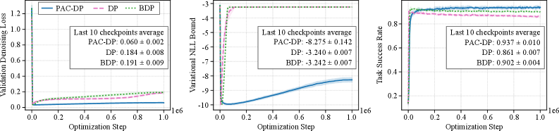
On the PushT task with 200 demonstrations (70% train/30% validation) trained for $10^6$ steps, DP and BDP show gradually increasing NPE (generalization degradation), while PAC-DP maintains a consistently low NPE throughout, converging to $0.060 \pm 0.002$—approximately a 67% reduction relative to DP's $0.184 \pm 0.008$. For variational NLL, DP/BDP quickly saturate near $-3.24$ (random Gaussian denoiser level), while PAC-DP maintains $-8.275 \pm 0.142$. For downstream success rate, PAC-DP converges to $93.7\% \pm 1.0\%$, while DP declines to $86.1\%$ and BDP to $90.2\%$.

Method	NPE ↓	Variational NLL ↓	Success Rate SR ↑
DP	0.184	-3.24	86.1%
BDP	0.191	-3.24	90.2%
PAC-DP	0.060	-8.275	93.7%

4.2 Robomimic Benchmark and Low-Data Evaluation

Across Lift, Can, Square, Transport, and ToolHang tasks with 200 demonstrations, PAC-DP achieves the lowest NPE and tightest NLL across all tasks. For success rate, on the challenging ToolHang task PAC-DP reaches 73.8% vs. DP's 40.1% and BDP's 54.4%. In low-data evaluation (20/40/80/200 demonstrations), PAC-DP shows the largest advantage at 20 demonstrations—ToolHang improves from 64.3% (DP) to 85.8% (PAC-DP, 200 demos).

Task	#Demos	DP SR	BDP SR	PAC-DP SR
PushT	20	48.1%	49.5%	54.9%
PushT	200	90.1%	92.6%	95.6%
Can	20	78.1%	86.5%	90.6%
ToolHang	200	64.3%	72.0%	85.8%

Ablation shows BDP (Bayesian parameterization without PAC-Bayes regularization) slightly improves success rate over DP but not in NPE/NLL—only PAC-DP leads across all metrics, confirming that the combination of Bayesian parameterization and PAC-Bayesian regularization is needed to maximize performance. Hyperparameter sensitivity analysis shows PAC-DP is stable across $\lambda \in \{10^{-5}, 10^{-6}\}$ and $\rho \in \{-3.5, -4.0, -4.5, -5.0\}$, not relying on fine tuning.

5. Limitations

• Prior selection: the current approach uses a fixed Gaussian prior; future work should investigate data-dependent priors for tighter PAC-Bayes bounds.
• Bounded loss assumption: the PAC-Bayes-kl inequality assumes bounded loss, while the denoising loss is theoretically unbounded; though it rapidly drops below 1 in practice making clipped and original objectives nearly identical, a theoretical gap remains.
• Computational overhead: Bayesian parameterization adds sampling overhead per forward pass; while training time increase is modest, it still impacts real-time inference scenarios.

6. Conclusion

PAC-DP models the diffusion policy as a Bayesian neural network and derives a training objective from the PAC-Bayes generalization bound that couples the empirical denoising loss with a KL-divergence regularizer, establishing a principled connection between statistical learning theory and diffusion policy optimization. Experiments show PAC-DP outperforms standard DP in denoising accuracy, variational NLL, and task success rate, with the largest improvements in low-data and challenging tasks—ToolHang with 200 demos improves from 64.3% to 85.8%. Ablation confirms gains stem primarily from PAC-Bayes regularization rather than Bayesian parameterization alone. Real-world Franka deployment validates sim-to-real transfer. The core insight: diffusion policy generalization cannot be guaranteed by the denoising objective alone—the PAC-Bayes bound tells us that a good policy must not only denoise accurately on training data, but its parameter distribution must remain simple, with deviations from the prior sufficiently supported by data.

flowchart TD
    A["Training data S = {z_i}"] --> B["Forward diffusion: x_t = sqrt(a_t) x_0 + sqrt(1-a_t) epsilon"]
    B --> C["Bayesian noise prediction network epsilon_w(x_t, t, o)"]
    D["Prior P(w) = N(0, sigma^2)"] --> E["KL divergence D_KL(Q || P)"]
    F["Posterior Q(w) = N(mu, diag(sigma^2))"] --> G["Reparameterization: w = mu + sigma * xi"]
    G --> C
    C --> H["Empirical denoising risk R_hat(Q)"]
    H --> I["PAC-DP objective: R_hat + KL regularization"]
    E --> I
    I --> J["SGD update posterior params mu, rho"]
    J --> F
    K["Inference: mean mu or sampling"] --> L["DDIM iterative denoising generates actions"]