PAPER DEEP DIVE
StreamSplat: Streaming Feed-Forward 3D Gaussian Splatting
Feed-forward 3D Gaussian Splatting enables efficient novel-view synthesis without per-scene optimization, but most existing methods assume a fixed set of context views and process them jointly. This limits their applicability to online scenarios where calibrated views arrive sequentially and the scene must be updated causally. We present \emph{StreamSplat}, a streaming feed-forward 3DGS framework that incrementally maintains a persistent geometry-grounded scene state and decodes it into renderable 3D Gaussians after each input chunk. StreamSplat centers on a \textbf{Voxel-Aligned Causal Cache (VACC)}, which stores historical 3D tokens in a memory-bounded voxel structure so that memory grows with explored scene geometry rather than stream length. To better reuse history during causal prediction, we introduce \textbf{History-Projected Depth Anchoring (HPDA)} to project cached geometry as depth guidance for current cost-volume estimation, and \textbf{Cache-Guided Feature Injection (CGFI)} to inject cached latent evidence into Gaussian-token regression. Experiments on DL3DV, RealEstate10K, and ScanNet show that StreamSplat remains competitive with state-of-the-art feed-forward 3DGS methods under sparse causal inputs, despite not using future views or full-scene context. More importantly, it scales to long input streams with 256, 512, and 1024 views where fixed-view baselines run out of memory, yielding sustained improvements in novel-view synthesis quality as more observations arrive. The code will be made publicly available upon acceptance.
One-Line Summary
StreamSplat proposes a streaming feed-forward 3DGS framework where a Voxel-Aligned Causal Cache (VACC) binds memory growth to explored scene geometry rather than stream length, sustaining novel-view synthesis quality improvements at 1024-view streaming inputs while all fixed-view baselines collapse from OOM beyond 128 views.
1. Background and Motivation
Novel-view synthesis (NVS) aims to reconstruct a 3D scene from observed images and render photorealistic views from novel viewpoints. 3D Gaussian Splatting (3DGS) has made explicit radiance-field reconstruction substantially more efficient through anisotropic Gaussian primitives and differentiable rasterization. Owing to its high rendering quality and real-time rasterization, 3DGS has become an increasingly attractive representation for AR/VR interaction, robotic perception, autonomous navigation, and other applications requiring spatially consistent visual understanding.
However, standard 3DGS still requires per-scene optimization to fit Gaussian parameters for each new scene. Feed-forward 3DGS methods (pixelSplat, MVSplat, DepthSplat, AnySplat, TokenSplat) seek to remove this optimization by learning to directly predict Gaussian scene representations from input images. These methods have made significant progress under fixed-view settings, but they all share a fundamental assumption: all context views are available before inference and processed jointly.
This assumption breaks in streaming scenarios. In online applications such as robot navigation and AR/VR interaction, calibrated views arrive frame by frame, and the scene must be updated causally—the model cannot wait for all observations before starting reconstruction but needs to output a renderable scene estimate as new observations arrive. This raises two core challenges: (1) the model needs a persistent memory that is spatially meaningful rather than merely temporal; and (2) incremental reconstruction must avoid accumulating local errors, since streaming inputs with limited overlap, occlusion, or weak texture can introduce incorrect geometry that subsequently affects reconstruction.
StreamSplat is designed to address these challenges. Its core idea: replace frame-level memory with a voxel-aligned 3D cache so historical information is indexed in space rather than accumulated in time; use History-Projected Depth Anchoring (HPDA) and Cache-Guided Feature Injection (CGFI) to feed cached geometric and appearance evidence back into current-frame depth estimation and Gaussian prediction, forming a geometry-grounded streaming reconstruction loop.
2. Preliminaries
Understanding StreamSplat requires two foundational concepts. First is the feed-forward 3DGS pipeline. Given calibrated context views $\{I_i, C_i\}_{i=1}^N$, the backbone converts images and camera parameters into 3D tokens:
$$\{I_i, C_i\}_{i=1}^N \rightarrow \{(p_j, f_j)\}_{j=1}^M \tag{2}$$
where $p_j$ is a world-space token position and $f_j$ is its latent feature. With a $4\times$ downsampled feature grid, the token count is $M = NHW/16$. Token positions are obtained through cost-volume-based depth estimation: for each reference view, the backbone samples depth candidates $\{d_k\}_{k=1}^D$, warps source-view features onto the reference image plane at each candidate depth, constructs a plane-sweep cost volume via dot-product correlations, and predicts a depth probability distribution through a U-Net decoder. The expected depth is:
$$\hat{d}_i(u) = \sum_{k=1}^D P_i(k \mid u) d_k \tag{3}$$
Second is the streaming reconstruction formulation. Given a calibrated view stream $\mathcal{V} = \{(I_t, C_t)\}_{t=1}^N$, the model at step $t$ consumes the current observation $(I_t, C_t)$ and historical cache $\mathcal{H}_{t-1}$, outputting newly predicted tokens $\mathcal{T}_t$, the updated cache $\mathcal{H}_t$, and the current Gaussian scene $\mathcal{G}_t$:
$$(\mathcal{T}_t, \mathcal{H}_t, \mathcal{G}_t) = F_\theta(I_t, C_t, \mathcal{H}_{t-1}) \tag{1}$$
This formulation gives the model an "anytime reconstruction" property: online applications may decode the current scene immediately after each chunk, while offline evaluation can decode only after the final context view. StreamSplat is built on ReSplat's feed-forward Gaussian reconstruction pipeline and DepthSplat's image encoder and geometry prediction backbone.
3. Methodology
3.1 Voxel-Aligned Causal Cache (VACC)
VACC is the persistent 3D memory of StreamSplat. At each streaming step, the base framework produces current 3D tokens $\{(p_j, f_j)\}$ from newly observed views, and VACC stores these tokens in a spatially indexed cache so historical evidence can be reused without retaining all past images or feature maps.
For each incoming token $m_\ell = (p_\ell, f_\ell)$, VACC first voxelizes the token position with voxel size $\Delta$ and assigns it to voxel $b_\ell$. The update is performed independently within voxel $b_\ell$. Each voxel stores at most $K$ pivot tokens, where each pivot summarizes a local appearance mode using an aggregated token state, a confidence weight, and a high-confidence seed feature. The confidence weight is the peak of the depth probability distribution:
$$\omega_\ell = \max_k P_i(k \mid u)$$
Low-confidence tokens ($\omega_\ell < \tau_{\text{conf}}$, set to $\tau_{\text{conf}} = 0.3$) are ignored to avoid polluting the long-term cache. When the voxel is not full, the token is directly inserted; when the voxel already contains $K$ pivots, the incoming token is added to the candidate set and the most similar pair is merged:
$$\mathcal{H}_{b_\ell}' = \begin{cases} \mathcal{H}_{b_\ell} \cup \{m_\ell\}, & n_{b_\ell} < K \\ \operatorname{MergeClosest}(\mathcal{H}_{b_\ell} \cup \{m_\ell\}), & n_{b_\ell} = K \end{cases} \tag{4}$$
MergeClosest selects the two tokens $m_0$ and $m_1$ with the highest cosine similarity between their features and replaces them with a confidence-weighted merged token:
$$p_\star = \frac{\omega_0 p_0 + \omega_1 p_1}{\omega_0 + \omega_1}, \quad f_\star = \frac{\omega_0 f_0 + \omega_1 f_1}{\omega_0 + \omega_1}, \quad \omega_\star = \max(\omega_0, \omega_1) \tag{5}$$
Experiments use $K=4$ and $\Delta=0.04$ (in world units). Because the voxel size is sufficiently small, tokens assigned to the same voxel are spatially close and usually correspond to the same local region, so within-voxel merging preserves fine geometric detail while removing redundant observations. Crucially, since VACC stores at most $K$ pivots per occupied voxel, memory grows with explored scene volume and voxel resolution, rather than with stream length.
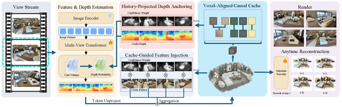
Figure 2: Overview of StreamSplat. The view stream is processed chunk by chunk: VACC maintains a geometry-grounded 3D history memory, HPDA projects cached geometry into current views as depth anchors, and CGFI reuses cached features to condition Gaussian-token regression.
3.2 History-Projected Depth Anchoring (HPDA)
HPDA uses the cached 3D history as geometric guidance for current views. The previous cache $\mathcal{H}_{t-1}$ is projected into each current view:
$$(D_\mathcal{H}^v, \Omega_\mathcal{H}^v, F_\mathcal{H}^v) = \mathcal{P}(\mathcal{H}_{t-1}, C_v) \tag{6}$$
where $C_v$ is the camera parameter of view $v$, and $D_\mathcal{H}^v$, $\Omega_\mathcal{H}^v$, $F_\mathcal{H}^v$ denote the projected cache depth, confidence weight, and confidence-weighted feature maps. For valid cache pixels, HPDA converts the projected cache depth into a confidence-aware Gaussian anchor over depth candidates:
$$P_\mathcal{H}^v(k, u) = \Omega_\mathcal{H}^v(u) \exp\left(-\frac{[d_k - \mu_\mathcal{H}^v(u)]^2}{2[\sigma_\mathcal{H}^v(u)]^2}\right) \tag{7}$$
where $\mu_\mathcal{H}^v(u) = D_\mathcal{H}^v(u)$ and variance $\sigma_\mathcal{H}^v(u) = \sigma_0 + \lambda_\sigma(1 - \Omega_\mathcal{H}^v(u))$. High-confidence cached geometry produces a sharper anchor, while uncertain cached observations produce a broader one. HPDA fuses this anchor with the cost volume's depth probability and renormalizes:
$$P^v(k \mid u) = \frac{P_i(k \mid u) + \gamma_d P_\mathcal{H}^v(k, u)}{\sum_{k'=1}^D [P_i(k' \mid u) + \gamma_d P_\mathcal{H}^v(k', u)]} \tag{8}$$
The cache-anchor strength $\gamma_d$ is a learnable scalar optimized jointly with the network rather than a manually tuned hyperparameter—the model itself decides how much to rely on cached geometry. HPDA thus lets current views reuse reliable historical geometry while still allowing the cost volume to revise uncertain cached structure.
3.3 Cache-Guided Feature Injection (CGFI)
CGFI complements HPDA by reusing historical appearance and latent evidence during Gaussian-token regression. The projected cache feature map $F_\mathcal{H}^v$ contains feature evidence accumulated from previous chunks. CGFI attenuates the cache feature by current uncertainty—pixels with high current confidence already have reliable local evidence:
$$\widehat{F}_\mathcal{H}^v(u) = (1 - \omega^v(u)) F_\mathcal{H}^v(u) \tag{9}$$
The attenuated cache feature is concatenated with the current token feature and aggregated by a 2D U-Net:
$$\widetilde{f}^v(u) = \Phi_{\text{agg}}\left(\operatorname{Concat}(f^v(u), \widehat{F}_\mathcal{H}^v(u))\right) \tag{10}$$
This way CGFI injects historical scene evidence only where it is useful, helping the model reduce local ambiguity without introducing an additional temporal feature memory. Predicted tokens are then passed to VACC for causal cache update, closing the streaming reconstruction loop.
3.4 Gaussian Decoder and Training Loss
The final scene representation is obtained by decoding cache-enhanced 3D tokens into explicit Gaussian primitives. Token 3D positions are used directly as Gaussian centers, and a lightweight two-layer MLP maps each aggregated feature to remaining Gaussian parameters (opacity, color coefficients, scale, rotation). During training, the decoder is applied to concatenated gradient-retaining tokens from all chunks for end-to-end rendering supervision; during inference, it is applied to the final fused cache, enabling the current streaming state to be converted into renderable 3D Gaussians at any time.
The training loss combines MSE and LPIPS:
$$\mathcal{L}_{\text{render}} = \sum_r \left[\text{MSE}(\hat{I}_r, I_r) + \lambda_{\text{LPIPS}} \ell_{\text{LPIPS}}(\hat{I}_r, I_r)\right] \tag{11}$$
flowchart LR
    subgraph INPUT["Input Stream"]
        IC["Image Chunk
(I_t, C_t)"]
    end
    subgraph CACHE["VACC: Voxel Cache"]
        VT["Voxelize tokens
at delta=0.04"]
        VT --> MF["MergeClosest
K=4 pivots/voxel"]
        MF --> HC["Historical Cache H_t"]
    end
    subgraph GUIDE["Cache-Guided Prediction"]
        HP["HPDA: project cache
to depth anchors"]
        CG["CGFI: inject cache
features at uncertain
pixels"]
        HP --> DE["Cost Volume
+ depth estimation"]
        CG --> GR["Gaussian-token
regression"]
    end
    IC --> DE
    HC --> HP
    HC --> CG
    DE --> GR
    GR -->|new tokens| VT
    GR -->|Gaussians| OUT["Renderable
3D Gaussians G_t"]
    style CACHE fill:#e8f0fe,stroke:#2563eb
    style GUIDE fill:#fef3c7,stroke:#d97706
    style INPUT fill:#dcfce7,stroke:#16a34a
Above: StreamSplat's streaming reconstruction loop. Input chunk to depth estimation (HPDA-guided) to Gaussian-token regression (CGFI-enhanced) to new tokens written into VACC to updated cache for next chunk.
4. Experimental Analysis
4.1 Competitiveness Under Sparse Inputs
With 24, 64, and 128 views, StreamSplat remains comparable to feed-forward 3DGS methods across DL3DV, RealEstate10K, and ScanNet. This is a more challenging setting—input is causal and sequential rather than globally available, so the model cannot rely on future views or full-scene context. Even under this constraint, StreamSplat achieves competitive quality.
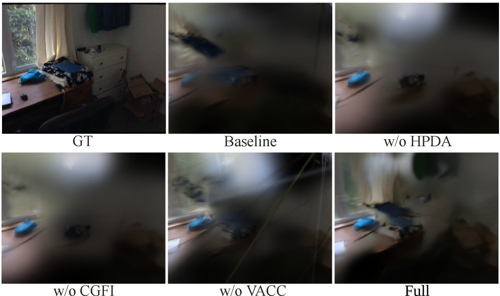
Table 1: Quantitative results on DL3DV, RealEstate10K, and ScanNet. "Mem." is peak GPU memory in GB; "OOM" denotes out-of-memory. Bold and underline mark the best and second-best per dataset and context length.
4.2 Long-Stream Scalability
Table 2 further evaluates whether longer context leads to better reconstruction quality. On ScanNet, as the input stream grows, StreamSplat's streaming design further supports 256, 512, and 1024 views, while all fixed-view baselines run out of memory under the same hardware and resolution. StreamSplat consistently improves as context increases from 256 to 512 and 1024 views: PSNR rises from 15.85 to 18.07, with corresponding gains in SSIM and LPIPS.
| Views | Method | PSNR ↑ | SSIM ↑ | LPIPS ↓ | Mem. (GB) ↓ |
|---|---|---|---|---|---|
| 256 | OF3GS | 12.48 | 0.483 | 0.659 | 23.1 |
| 256 | StreamSplat | 15.85 | 0.597 | 0.582 | 24.5 |
| 512 | OF3GS | 12.31 | 0.482 | 0.667 | 41.4 |
| 512 | StreamSplat | 16.98 | 0.637 | 0.568 | 44.7 |
| 1024 | OF3GS | - | - | - | OOM |
| 1024 | StreamSplat | 18.07 | 0.669 | 0.549 | 87.3 |
On DL3DV at 256 views, StreamSplat achieves 20.15 PSNR versus OF3GS's 14.00. On RealEstate10K at 256 views, StreamSplat achieves 19.18 versus OF3GS's 13.44. This contrast shows that the persistent cache not only enables long-sequence processing but also effectively accumulates additional observations into a higher-quality
| Dataset | Method | 24-view PSNR | 64-view PSNR | 128-view PSNR |
|---|---|---|---|---|
| DL3DV | DepthSplat | 13.41 | 15.02 | OOM |
| DL3DV | ReSplat | 14.48 | 16.80 | 19.10 |
| DL3DV | StreamSplat | 12.95 | 15.38 | 18.36 |
| RealEstate10K | ReSplat | 13.62 | 15.93 | 18.40 |
| RealEstate10K | StreamSplat | 13.03 | 14.94 | 17.84 |
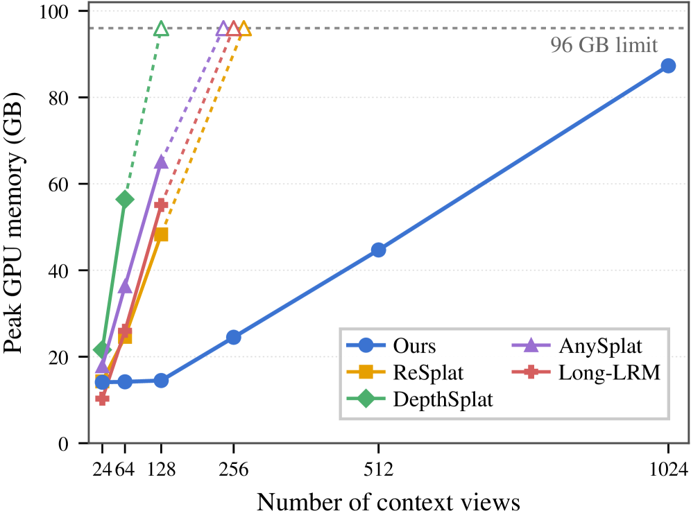
Figure 1: Peak GPU memory under increasing context lengths on ScanNet. Baseline memory grows rapidly with jointly processed views, while StreamSplat's chunk-wise processing and memory-bounded voxel cache stay far lower.
4.3 Ablation Studies
The ablation evaluates each module's contribution on ScanNet at 256 views. Removing VACC and replacing it with an append-all cache slightly improves the 256-view score (PSNR 16.14 vs 15.85) but spikes peak memory from 24.5GB to 41.3GB and OOMs at 512 views. VACC is thus an explicit accuracy-memory trade-off: trading 0.29dB for the ability to scale to 512 views. Removing HPDA drops PSNR from 15.85 to 14.61 and increases LPIPS from 0.582 to 0.613. Removing CGFI drops PSNR to 14.77 and increases LPIPS to 0.612. Both guidance modules also reduce peak memory—because they keep per-chunk predictions consistent with the cache, repeated observations of the same surface fall into the same voxels and are absorbed by within-voxel merging.
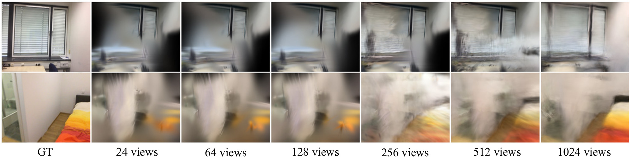
Table 2: Results at extended context lengths, with peak memory in GB. OF3GS is the only baseline that runs beyond 128 views.
5. Discussion
StreamSplat's core contribution lies in transforming 3DGS from a "one-shot all-views" paradigm to a "streaming causal accumulation" paradigm. VACC's voxel-aligned design is the key technical decision enabling this transformation: by indexing historical tokens in 3D space rather than in temporal sequences, memory growth is bound to explored scene geometry rather than stream length. This means a 1000-frame scene and a 100-frame scene covering the same physical space have similar cache sizes—a fundamental advantage impossible for fixed-view methods.
HPDA and CGFI embody the principle of "uncertainty-driven history reuse." HPDA uses confidence-aware Gaussian anchors to guide depth estimation—high-confidence history produces sharp anchors, low-confidence produces broad ones, allowing the cost volume to revise uncertain cached structure. CGFI attenuates cache features by current uncertainty—injecting historical information only at pixels where current prediction is unreliable, avoiding redundant interference in regions with sufficient local evidence. This adaptive mechanism makes StreamSplat non-inferior to all-view methods under sparse inputs while continuing to benefit under dense inputs.
From an application perspective, StreamSplat's "anytime reconstruction" property has direct value for robotic perception and autonomous navigation. A robot can incrementally build a scene representation during navigation, obtaining a renderable 3D Gaussian scene after each input chunk rather than waiting for a complete observation sequence. The 143ms end-to-end latency (6.98 FPS) approaches real-time requirements, and the memory-bounded property enables long-duration operation.
6. Limitations
Accuracy-memory trade-off: VACC trades 0.29dB of accuracy for memory scalability through within-voxel merging. In scenes with highly complex geometry where the same local region requires preserving multiple appearance modes (e.g., reflections, transparent surfaces), the $K=4$ pivot limit may be insufficient. The paper does not discuss how to adaptively choose voxel size $\Delta$ and pivot count $K$ for different scene complexities.
Calibration dependency and static-scene assumption: StreamSplat requires a calibrated view stream (known camera intrinsics and extrinsics), which is not always satisfied in real robotic scenarios. Additionally, the paper focuses on static-scene novel-view synthesis and does not handle dynamic objects. While Wu et al. (2026)'s same-named StreamSplat extends streaming Gaussian reconstruction to dynamic scenes, this work itself does not support dynamic content. Finally, under sparse inputs (24 views), StreamSplat's PSNR on DL3DV (12.95) is below DepthSplat (13.41) and ReSplat (14.48), indicating that introducing cached information with very few views may still have negative effects requiring further analysis.
7. Conclusion and Outlook
StreamSplat proposes a streaming feed-forward 3DGS framework where VACC stores historical tokens in a memory-bounded voxel cache, making scene state scale with explored geometry rather than stream length. HPDA and CGFI feed cached geometric and appearance evidence back into current-frame depth estimation and Gaussian prediction, forming a geometry-grounded streaming reconstruction loop. On DL3DV, RealEstate10K, and ScanNet, StreamSplat remains competitive under sparse causal inputs and, more importantly, scales to long input streams (256, 512, 1024 views) where fixed-view baselines run out of memory, with quality consistently improving as more observations arrive.
From a broader perspective, StreamSplat represents a paradigm shift in 3DGS from "batch reconstruction" to "online incremental reconstruction." The voxel-aligned cache design philosophy—compressing temporal dimensions into spatial dimensions—may inspire broader streaming 3D perception tasks such as streaming NeRF and online SLAM. Future work may explore: pose-free streaming reconstruction without calibration, dynamic-scene extensions, and real-time deployment on edge devices.
SOURCE LINKS