WilLaGS: Latent-Conditional 3D Appearance Fields for Robust Gaussian Splatting In-the-Wild

Paper metadata. Authors: Yuhao Bai (Nanjing University), Qianqiu Tan (Nanjing Agricultural University), Lilong Chen, Huanhuan Lv, and Lijun Chen (Nanjing University, corresponding author). arXiv:2608.28240v1 [cs.CV], submitted 28 August 2026. Paper: https://arxiv.org/abs/2608.28240. Code status: no public implementation released — the paper contains no repository link, and a GitHub search only surfaces an empty organization profile (WilLaGS/WilLaGS) with no source code.

One-sentence summary. WilLaGS replaces the discrete per-image appearance embeddings used by prior in-the-wild 3DGS methods with a β-VAE generative latent space that conditions a Tri-Plane 3D appearance field for spatially-varying illumination, and adds a self-supervised teacher–student perceptual mask to exclude transient objects — reaching state-of-the-art reconstruction on Photo Tourism and NeRF-OSR (25.84 dB PSNR on Sacré-Cœur, +2.28 dB over AsymGS) while training in 0.9 GPU-hours and rendering at 58 FPS.

1. Research Background and Motivation

Novel view synthesis from unconstrained photo collections is a building block for VR/AR, robotics perception, and digital content creation. 3D Gaussian Splatting (3DGS) made this practical in the lab: its explicit Gaussian primitives plus a differentiable tile-based rasterizer deliver fast convergence and real-time rendering. But 3DGS was designed for static, consistently-lit scenes, and in-the-wild collections violate both assumptions at once. Tourist photos of the same landmark are shot at different hours, under different weather, and are riddled with transient occluders — pedestrians, cars, scaffolding.

The paper frames this as two coupled challenges. First, severe appearance variation breaks photometric consistency across views. Second, pervasive transient objects occlude the static scene. Together they violate the multi-view consistency assumption of 3DGS and produce the familiar failure modes: ghosting, blur, and distorted geometry.

Existing work treats these two problems separately, and each side has a structural weakness. For appearance, most methods (NeRF-W, Ha-NeRF, WildGaussians and successors) attach an independently optimized embedding to each training image. Such discrete embeddings are fundamentally ill-suited to continuous real-world illumination: they memorize the appearance of their own image rather than learning a generalizable manifold, and a single global code cannot express spatially-varying effects like localized highlights or cast shadows. For transients, prior methods either pay for auxiliary segmentation networks and extra supervision, or rely on pretrained detectors tied to specific object categories, and pixel-level consistency masks mistake illumination shifts for transients.

WilLaGS's thesis is that both problems can be solved inside one self-supervised framework: a generative appearance model learns the continuous manifold of global scene appearance, a latent-conditioned 3D field converts that global code into local, spatially-varying illumination, and a teacher–student perceptual mask uses the model's own temporally-smoothed consensus to identify what does not belong to the static scene. No external detectors, no manual masks, no extra supervision.

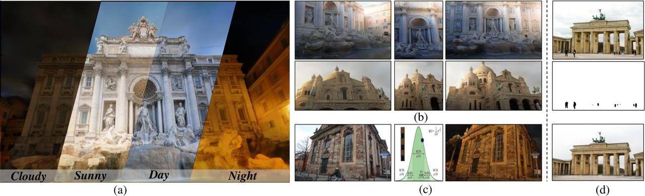
Figure 1: WilLaGS capabilities from the paper teaser: (a) diverse appearance rendering, (b) strict multi-view consistency, (c) unconditional novel appearance synthesis, and (d) robust transient object removal.

2. Preliminaries: 3D Gaussian Splatting

3DGS represents a scene as a set of anisotropic Gaussian primitives, each with a center $\mu_{i}\in\mathbb{R}^{3}$, a positive semi-definite covariance $\Sigma_{i}\in\mathbb{R}^{3\times 3}$, an opacity $\alpha_{i}$, and a view-dependent color parameterized by spherical harmonics. Rendering projects the Gaussians to the image plane, sorts them by depth, and alpha-composites them tile by tile. The color of a pixel is

$$C=\sum_{i=1}^{N}c_{i}\,\alpha_{i}^{\prime}\prod_{j=1}^{i-1}(1-\alpha_{j}^{\prime}),\qquad \alpha_{i}^{\prime}=\alpha_{i}\cdot\exp\left(-\tfrac{1}{2}(x-\mu_{i}^{\prime})^{T}(\Sigma_{i}^{\prime})^{-1}(x-\mu_{i}^{\prime})\right) \tag{1}$$

where $c_{i}$ is the view-dependent color of Gaussian $i$ and $\mu_{i}^{\prime},\Sigma_{i}^{\prime}$ are its projected 2D mean and covariance. In in-the-wild variants, the SH color is typically replaced by an appearance-conditioned decoder — WilLaGS keeps the Gaussian backbone but rebuilds exactly this color pathway.

3. Method

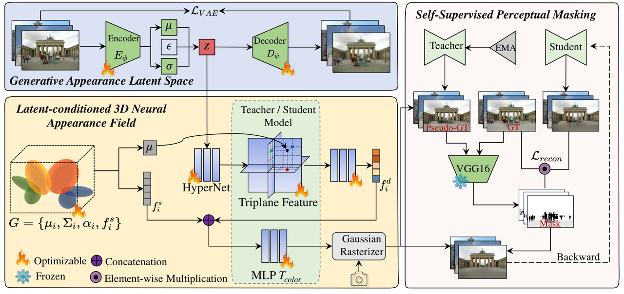
Figure 2: Framework overview. A β-VAE learns a generative appearance manifold; conditioned on the latent code z, a Tri-Plane 3D appearance field modulates spatially-varying local illumination; a self-supervised teacher–student perceptual mask suppresses transient objects.

3.1 Generative appearance latent space (β-VAE)

Instead of one free embedding per image, WilLaGS learns a continuous latent space with a β-Variational Autoencoder. An encoder $E_{\phi}$ maps each image $I_{j}$ to a posterior $q_{\phi}(z|I_{j})=\mathcal{N}(\mu_{j},\sigma_{j}^{2})$, and a decoder $D_{\psi}$ reconstructs the image from a sampled code $z_{j}$. Training optimizes the weighted ELBO:

$$\mathcal{L}_{\text{VAE}}=\mathcal{L}_{\text{recon}}(I_{j},\hat{I}_{j})+\beta\cdot D_{\text{KL}}\big(q_{\phi}(z|I_{j})\,\|\,p(z)\big) \tag{2}$$

with the prior $p(z)=\mathcal{N}(0,I)$. The key design choice is $\beta>1$ (the paper sets $\beta=2$). A larger β tightens the information bottleneck: the encoder is forced to discard redundant correlations and high-frequency, image-specific noise, and to keep only the essential global factors — illumination, weather, tone. The result is a compact, smooth, statistically structured manifold that generalizes beyond the training images instead of memorizing them, and that is directly samplable for generation. Implementation-wise the latent dimension is 64.

3.2 Latent-conditioned 3D appearance field

A global code alone cannot produce a localized shadow on one façade while leaving another in sun. WilLaGS therefore expands each latent code into a spatially-aware 3D field via a hypernetwork $H$: the code $z_{j}\in\mathbb{R}^{d}$ is mapped to the parameters $\Theta_{field}(z_{j})$ of a lightweight neural field, realized as three orthogonal Tri-Plane feature planes:

$$\{P_{XY},P_{XZ},P_{YZ}\}=\text{Hypernetwork}(z_{j}) \tag{3}$$

Each plane has spatial resolution $64\times 64$ and 32 channels, so a different latent code literally rewrites the entire 3D appearance field. To query it, a Gaussian at $\mu_{i}$ is normalized to $\mu_{i}^{\prime}\in[-1,1]^{3}$ by the scene bounds, projected onto the three planes, and sampled with bilinear interpolation:

$$f_{XY}=\text{Sample}(P_{XY},(x_{i}^{\prime},y_{i}^{\prime})),\quad f_{XZ}=\text{Sample}(P_{XZ},(x_{i}^{\prime},z_{i}^{\prime})),\quad f_{YZ}=\text{Sample}(P_{YZ},(y_{i}^{\prime},z_{i}^{\prime})) \tag{4}$$

The three sampled vectors pass through a small MLP $T_{\theta}$ to yield the dynamic appearance feature of that Gaussian:

$$f_{i}^{d}=T_{\theta}(f_{XY},f_{XZ},f_{YZ}) \tag{5}$$

Because the query is coordinate-based, every Gaussian receives illumination information that is both conditioned on the global code and specific to its 3D location — exactly the spatially-varying local illumination that global embeddings miss.

To keep geometry and material stable while lighting changes, the authors adopt an appearance-disentanglement strategy inspired by GS-W. Each Gaussian additionally carries a learnable intrinsic feature $f_{i}^{s}$ encoding material-like attributes (albedo, reflectance) that stay invariant across illumination conditions. A lightweight fusion decoder combines everything into the final view-dependent color:

$$C=T_{\text{color}}(f_{i}^{d},f_{i}^{s},d) \tag{6}$$

where $d$ is the viewing direction. Both $f_{i}^{d}$ and $f_{i}^{s}$ are 32-dimensional; the hypernetwork generator and $T_{\text{color}}$ are lightweight 3-layer MLPs with ReLU activations. The split means the latent code can modulate local lighting without touching intrinsic material properties — a controllable, disentangled appearance representation.

3.3 Self-supervised transient masking

Figure 3: Why perceptual, not pixel-level, differences: pixel diffs fire on illumination shifts, perceptual diffs isolate structural/content inconsistency caused by transients.

The masking module has two moving parts. First, a teacher–student pair with identical architecture (appearance field plus color decoder). The student is trained normally; the teacher weights are an exponential moving average of the student's:

$$W_{T}\leftarrow\tau W_{T}+(1-\tau)W_{S} \tag{7}$$

Because the EMA integrates the student over time, the teacher converges to a temporally smoothed consensus of the static scene and its average appearance — high-frequency temporal variation caused by transient objects is averaged out. During training the teacher renders a pseudo-ground-truth reference $\hat{I}_{pseudo}$ for the current view.

Second, the mask itself. A naive pixel difference between ground truth and the teacher reference would flag every illumination shift as a transient (Fig. 3), so the comparison happens in perceptual feature space: both images pass through a frozen pretrained VGG, and L1 differences are taken across layers $\phi_{l}\in\{\texttt{relu1\_2},\texttt{relu2\_2},\texttt{relu3\_3}\}$, averaged over channels and summed over layers:

$$D_{\text{perceptual}}(p)=\sum_{l}\|\phi_{l}(I_{gt})(p)-\phi_{l}(\hat{I}_{pseudo})(p)\|_{1} \tag{8}$$

Thresholding yields a binary static mask:

$$M_{\text{static}}(p)=\big(D_{\text{perceptual}}(p)\lt\lambda_{mask}\big) \tag{9}$$

with $\lambda_{mask}=0.85$ in all experiments. Low-discrepancy pixels are treated as consistent static background; high-discrepancy regions — the transients — are excluded from supervision. Because VGG features are comparatively insensitive to global tone shifts, the mask targets structural and content-level inconsistency rather than lighting.

3.4 Training objective

The reconstruction loss applies L1 and D-SSIM only inside the static mask:

$$\mathcal{L}_{\text{recon}}=\lambda_{L1}\,\mathcal{L}_{1}(I_{\text{render}}\odot M_{\text{static}},I_{\text{gt}}\odot M_{\text{static}})+\lambda_{\text{DSSIM}}\,\mathcal{L}_{\text{DSSIM}}(I_{\text{render}}\odot M_{\text{static}},I_{\text{gt}}\odot M_{\text{static}}) \tag{10}$$

and the total loss couples it with the VAE objective:

$$\mathcal{L}_{\text{total}}=\mathcal{L}_{\text{recon}}+\lambda_{VAE}\,\mathcal{L}_{\text{VAE}} \tag{11}$$

with $\lambda_{L1}=0.8$, $\lambda_{\text{DSSIM}}=0.2$, and $\lambda_{VAE}=0.01$. The whole framework is PyTorch + Adam, trained 30k steps on a single NVIDIA RTX 3090.

flowchart TD
    A["In-the-wild image collection
lighting, weather, transients"] --> B["β-VAE encoder E_phi
maps each image to a latent distribution"]
    B --> Z["Global appearance latent code z"]
    Z --> H["Hypernetwork H"]
    H --> TP["Tri-Plane feature planes
P_XY, P_XZ, P_YZ"]
    G["Gaussian centers mu_i
normalized to scene bounds"] --> S["Bilinear sampling
f_XY, f_XZ, f_YZ"]
    TP --> S
    S --> T["Small MLP T_theta"]
    T --> FD["Dynamic feature f_i_d
spatially varying illumination"]
    FD --> C["Fusion decoder T_color
inputs: f_d, f_s, view direction d"]
    IS["Learnable intrinsic feature f_i_s
albedo and reflectance"] --> C
    C --> R["Rendered image I_render"]
    R --> L["Masked L1 + D-SSIM loss, Eq. 10"]
    GT["Ground truth I_gt"] --> VGG["Frozen VGG perceptual features
relu1_2, relu2_2, relu3_3"]
    TE["EMA teacher W_T, Eq. 7
slow consensus renderer"] --> PS["Pseudo reference I_pseudo"]
    PS --> VGG
    VGG --> DM["Perceptual difference map D_perceptual"]
    DM --> MK["Threshold lambda_mask
binary static mask M_static"]
    MK --> L
    L --> UPD["Update student weights W_S"]
    UPD --> EMA["W_T = tau W_T + 1-tau W_S"]
    EMA --> TE

Pipeline of WilLaGS: the β-VAE code conditions a Tri-Plane appearance field, and the EMA teacher's perceptual disagreement with the ground truth gates which pixels supervise the student.

4. Experiments

4.1 Setup

Evaluation uses two standard in-the-wild benchmarks: Photo Tourism (PT) with the large-scale landmarks Brandenburg Gate, Trevi Fountain, and Sacré-Cœur, and NeRF-OSR with four outdoor scenes (europa, lwp, st, stjohann) exhibiting strong illumination and weather variation. Baselines span NeRF-based methods (NeRF-W, Ha-NeRF, CR-NeRF, K-Planes) and 3DGS-based methods (3DGS, SWAG, GS-W, Splatfacto-W, AsymGS, DeSplat, WildGaussians). Metrics are PSNR, SSIM, and LPIPS; following the NeRF-W protocol, the appearance latent is optimized on the left half of each test image and quality is measured on the unseen right half. Training time and rendering FPS are also reported.

4.2 Quantitative comparison

Method	Sacré-Cœur PSNR↑	SSIM↑	LPIPS↓	Trevi PSNR↑	SSIM↑	LPIPS↓	Brandenburg PSNR↑	SSIM↑	LPIPS↓	GPU hrs / FPS
NeRF-W	19.20	0.808	0.192	18.97	0.698	0.265	24.17	0.891	0.167	42 / <1
Ha-NeRF	20.02	0.801	0.171	20.18	0.691	0.223	24.04	0.887	0.139	35 / <1
CR-NeRF	22.07	0.823	0.152	21.48	0.712	0.207	26.53	0.900	0.106	31 / <1
K-Planes	20.61	0.768	0.352	22.69	0.726	0.351	23.23	0.865	0.282	0.3 / <1
3DGS	17.49	0.828	0.217	17.35	0.674	0.300	19.80	0.883	0.179	0.4 / 105
SWAG*	21.16	0.860	0.185	23.10	0.815	0.208	26.33	0.929	0.139	0.8 / 15
GS-W	22.23	0.836	0.291	22.93	0.773	0.217	26.86	0.921	0.243	2.0 / 50
Splatfacto-W	22.52	0.867	0.169	22.64	0.762	0.229	26.75	0.926	0.143	1.1 / 40
AsymGS	23.56	0.877	0.169	23.91	0.785	0.223	28.49	0.928	0.139	5.6 / 47
DeSplat	20.14	0.868	0.178	23.31	0.775	0.226	25.04	0.920	0.142	2.4 / 53
WildGaussians	22.71	0.859	0.173	23.70	0.768	0.228	27.36	0.927	0.141	7.8 / 73
WilLaGS (Ours)	25.84	0.891	0.164	24.54	0.789	0.207	29.94	0.939	0.139	0.9 / 58

Table 1: Quantitative comparison on the Photo Tourism dataset (best results bolded; SWAG numbers taken from the original paper).

On PT, WilLaGS posts the best PSNR on all three scenes. The standout is Sacré-Cœur — 25.84 dB against AsymGS's 23.56 dB, a +2.28 dB leap on a scene notorious for extreme lighting diversity — plus the best SSIM everywhere and best or tied LPIPS. The efficiency column is equally telling: the full pipeline costs 0.9 GPU-hours per scene versus 5.6 for AsymGS and 7.8 for WildGaussians, while rendering at 58 FPS (only vanilla 3DGS and WildGaussians render faster, both with far lower quality).

Method	europa PSNR↑	SSIM↑	LPIPS↓	lwp PSNR↑	SSIM↑	LPIPS↓	st PSNR↑	SSIM↑	LPIPS↓	stjohann PSNR↑	SSIM↑	LPIPS↓
NeRF-W	20.00	0.699	0.347	19.61	0.616	0.445	20.31	0.607	0.438	21.23	0.667	0.426
Ha-NeRF	17.79	0.632	0.421	20.03	0.685	0.365	17.30	0.538	0.483	19.93	0.686	0.331
CR-NeRF	19.92	0.696	0.310	20.61	0.736	0.358	20.47	0.661	0.390	21.27	0.815	0.275
3DGS	17.71	0.728	0.311	15.41	0.686	0.337	16.09	0.667	0.356	16.17	0.744	0.289
GS-W	23.31	0.833	0.335	22.25	0.784	0.357	23.13	0.754	0.398	25.72	0.894	0.276
WildGaussians	20.82	0.724	0.393	22.12	0.791	0.289	19.90	0.695	0.375	22.77	0.881	0.184
WilLaGS (Ours)	24.38	0.843	0.216	23.36	0.818	0.230	23.43	0.763	0.267	25.55	0.906	0.161

Table 2: Quantitative results on NeRF-OSR. WilLaGS leads across all scenes on PSNR, SSIM, and LPIPS (stjohann PSNR within 0.17 dB of GS-W while ahead on the other two metrics).

On NeRF-OSR, WilLaGS wins every metric on three of four scenes and takes SSIM+LPIPS on the fourth (stjohann PSNR is 25.55 vs GS-W's 25.72). The LPIPS margins are large — on europa, 0.216 versus 0.335 for GS-W — indicating the gains are perceptual, not just pixel-wise.

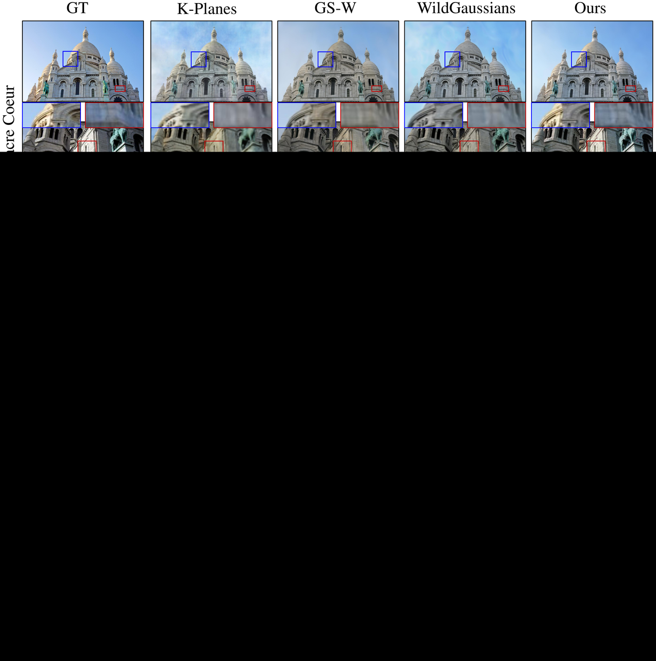
Figure 4: Qualitative comparison on PT. WilLaGS recovers crisp Brandenburg Gate pillars and Trevi Fountain façade carvings, and synthesizes localized shadows in Sacré-Cœur alcoves while suppressing ghosting.

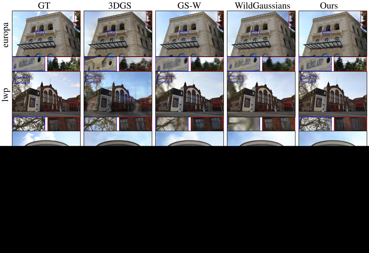
Figure 5: Qualitative comparison on NeRF-OSR. WilLaGS preserves high-frequency structure that baselines over-smooth: legible banner text (st) and fine tree branches (lwp), under complex outdoor lighting.

Qualitatively, baselines such as K-Planes and GS-W blur high-frequency structure, while WilLaGS recovers crisp architectural detail and, on NeRF-OSR, legible banner text and thin tree branches. Equally important, the latent-conditioned field produces genuine spatially-varying illumination — localized shadows and realistic lighting gradients on Sacré-Cœur — where prior methods collapse to flat global color shifts.

4.3 Ablations

Variant	PT PSNR↑	PT SSIM↑	PT LPIPS↓	OSR PSNR↑	OSR SSIM↑	OSR LPIPS↓
w/o VAE latent space (per-image embeddings)	22.15	0.835	0.197	21.54	0.802	0.233
w/o 3D appearance field (concat z with f_s)	25.05	0.853	0.191	23.02	0.817	0.235
w/o teacher–student mask	26.19	0.861	0.182	23.94	0.825	0.226
Full WilLaGS	26.77	0.873	0.170	24.18	0.832	0.218

Table 3: Ablation on key components, averaged over all scenes of PT and NeRF-OSR.

The ablations rank the components cleanly. Swapping the β-VAE for NeRF-W-style discrete per-image embeddings is catastrophic: −4.62 dB PSNR on PT and −2.64 dB on NeRF-OSR — independent deterministic embeddings overfit their own images and learn nothing generalizable. Replacing the Tri-Plane field with a plain concatenation of $z$ and $f_{i}^{s}$ costs about 1.7 dB on PT, and qualitatively flattens lighting into spatially-uniform shading (Fig. 6). Disabling the mask costs ~0.6 dB on average but produces severe ghosting and blurry floaters wherever transients are dense. Overhead is modest: ~933 MB of extra trainable VRAM (β-VAE ~66.64 MB, 3D field ~866.75 MB) plus a fixed ~528 MB for the frozen VGG-16.

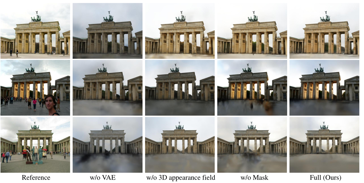
Figure 6: Qualitative ablations. Without the VAE latent space colors become inconsistent; without the 3D appearance field shadows turn unnatural and spatially uniform; without the self-supervised mask, ghosting artifacts dominate.

4.4 Applications

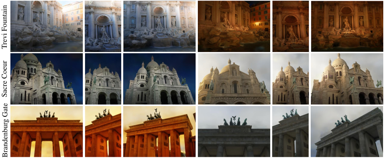
Figure 7: Multi-view appearance modeling — one latent code re-rendered along different camera trajectories stays geometrically and photometrically consistent.

Because the appearance model is generative rather than per-image, three applications fall out for free. First, appearance modeling and transfer: fixing a latent code $z$ re-renders the scene from arbitrary viewpoints under the corresponding lighting with strict multi-view consistency — sunlight hits the correct Trevi Fountain façades and casts geometrically consistent shadows across poses (Fig. 7). Second, appearance interpolation between two reference codes:

$$z_{\text{interp}}=(1-\alpha)z_{a}+\alpha z_{b},\qquad \alpha\in[0,1] \tag{12}$$

which sweeps smoothly from one condition to another (e.g., sunny to night) while preserving scene structure (Fig. 8a). Third, unconditional synthesis: since the β-VAE regularizes the latent space toward $p(z)=\mathcal{N}(0,I)$, sampling random $z\sim p(z)$ generates physically plausible new lighting and weather — night, sunset, overcast — with no reference image at all (Fig. 8b). That behavior is the strongest evidence that the model learned a structured generative manifold rather than a lookup table of training appearances.

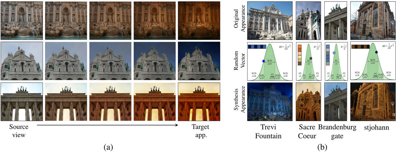
Figure 8: (a) Appearance interpolation from a fixed viewpoint between two latent codes; (b) novel appearance synthesis from random latent vectors sampled from the learned standard Gaussian prior.

5. Limitations

Dense occlusions remain hard (stated by the authors). The teacher–student mask suppresses inconsistent transient regions, but persistently dense occlusion — crowds that cover a façade for most views — still leaves too little static supervision for clean reconstruction, and the paper flags this explicitly.

No explicit physical interpretability (stated by the authors). The latent manifold is learned, not parameterized: there is no explicit sun direction, cloud cover, or exposure variable to control, which limits deterministic editing. The authors point to semantic control over the latent manifold and scaling to large scenes as future work.

Evaluation scope (my reading). Both benchmarks are landmark-scale photo collections; behavior on city-scale or indoor multi-room collections is untested, and each scene is trained independently, so cross-scene generalization of the appearance prior is not measured. The test-time protocol — optimizing the latent on the left half of each test image — is standard for this line of work but favors methods with a smooth latent space, worth keeping in mind when comparing the margins.

6. Conclusion

WilLaGS argues that in-the-wild 3DGS fails when appearance is modeled as a bag of independent embeddings, and fixes it at the representation level: a β-VAE learns a continuous, generative manifold of global appearance; a latent-conditioned Tri-Plane field turns each code into spatially-varying 3D illumination; and an EMA teacher's perceptual disagreement with the ground truth self-supervises transient removal. The combination delivers the best published numbers on Photo Tourism and NeRF-OSR at a fraction of the training cost (0.9 GPU-hours) with real-time 58 FPS rendering, and unlocks appearance transfer, interpolation, and unconditional synthesis as natural byproducts. With code not yet public, reproduction of the +2.28 dB Sacré-Cœur result is the field's next checkpoint.

7. Golden Quote

"Geometry stays put while appearance flows: WilLaGS gives one static scene a whole generative manifold of weathers — and lets a slow teacher decide, pixel by pixel, what actually belongs to the scene."