Dream-RSI: Recursive Self-Improvement through Evolving Worlds

Dream-RSI: Turning Discovery History into a Replayable World

Title: Dream-RSI: Recursive Self-Improvement through Evolving Worlds
Authors: Tong Zheng, Xidong Wu, Zheng Zhang, Zhankui He, Chaoyi Zhang, Benjamin Coleman, Ruoqiao Wei, Di Bai, Haolin Liu, Rui Liu, Xue Wang, Yue Zhuan, Wang-Cheng Kang, Renkai Xiang, Heng Huang, Xinwu Cheng, Yunsong Guo (17 authors)
Affiliations: Google, Google DeepMind, University of Maryland College Park, University of Virginia
arXiv: arXiv:2609.14858v1 [cs.CL] (14 Sep 2026)
Code status: the repository github.com/zhengkid/Dream-RSI exists, but its README marks the full codebase and the discovered programs as still being prepared; the project page is dream-rsi.com. The reproducible material therefore currently lives in the paper itself: Appendix B contains the complete online-exploration and replay-based policy-improvement prompts, and Appendix C contains the full source of the discovered Lasso-path solver.

One-Sentence Summary

Treat a finished discovery run as a replayable world model: candidate exploration policies "dream" over the recorded discovery tree, get scored and rewritten using only outcomes that are already stored, and the best-scoring version is redeployed online — which turns meta-level recursive self-improvement from expensive online trial and error into cheap offline simulation.

Background: Self-Improvement Bottlenecks at the Exploration Layer

The standard engine behind recursive self-improvement (RSI) is a discovery loop: an agent proposes candidate solutions, evaluates outcomes, absorbs feedback, and revises how it proposes next time. That loop has produced real results in algorithm design, open-ended mathematical optimization, systems design, and agent self-improvement, and those results feed back into more capable AI systems. As the targets get harder, discovery itself gets longer: a single search now routinely spans thousands of proposal–evaluation cycles. At that scale, what determines efficiency is no longer the quality of one proposal but the orchestration of exploration — which branch to deepen, how much compute to fan out in parallel, and when to stop.

Most existing systems rely on manually designed exploration strategies that stay fixed for the whole run. A fixed strategy cannot learn from accumulated discovery experience, so it may keep spending compute on directions that have already saturated. Recent work such as EvoX optimizes the exploration policy online during discovery, but runs into two structural bottlenecks. First, meta-level feedback is delayed and expensive: scoring a single candidate takes one execution, whereas scoring an exploration policy requires watching how it shapes many subsequent proposal–evaluation cycles. Second, the meta-policy space is vast, and a newly proposed policy may simply be bad, so many alternatives must be tried. Together these mean every candidate policy needs a long online rollout before it yields any useful signal, which is exactly why the self-improvement loop is hard to close at the exploration layer.

The authors' intuition is plain: with a fast, cheap simulator of discovery, many exploration policies could be evaluated before any expensive online deployment. Their observation is that completed discovery histories already provide such a simulator. Prior work treats past history either as static textual context stuffed back into the prompt or as training data for weight fine-tuning. But what a completed discovery process actually records is a structured tree of past exploration decisions together with their realized code-execution outcomes.

That tree is the same kind of object as a world model in model-based reinforcement learning. The Dreamer family learns a compact dynamics model from collected experience and improves its policy by imagining trajectories inside that model. A discovery tree is an already-realized empirical world model: every node's outcome is stored, so evaluating a different policy only requires revealing recorded branches in a different subset, a different order, with different parallel groupings and different stopping decisions — without rerunning the underlying coding agent or evaluator. Meta-policy improvement stops being expensive online trial and error and becomes a fast, simulation-based dreaming procedure.

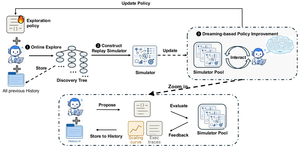
Figure 1: The Dream-RSI loop. (1) Online Explore — the current policy drives a coding agent to expand a discovery tree and log historical traces; (2) Construct Replay Simulator — the tree becomes a reusable simulator pool; (3) Dreaming-based Policy Improvement — the agent dreams up a large pool of alternative policies, feeds them into the simulator for rapid feedback, and redeploys the winner online.

On top of this, the paper introduces Dream-RSI: a lightweight orchestration layer makes exploration explicit and programmable (branching, parallel exploration, stopping) while leaving the underlying coding agent untouched, and a three-stage closed loop — online exploration, simulator construction, dreaming-based policy improvement — keeps re-deploying the improved policy so that new experience expands the simulator pool. Evaluation spans 8 scientific discovery tasks in 3 domains: algorithm engineering (Lasso regularization path), mathematical optimization (sum–difference, circle packing, autocorrelation inequalities), and GPU kernel engineering (four KernelBench tasks).

Preliminaries: Discovery Trees and the Shared Decision Interface

A discovery tree is rooted at $r$, the initial workspace state. Every non-root node $v$ has exactly one primary parent — the root or a previously created node — and that parent identifies where the attempt in $v$ begins: the discovery agent resumes the parent's saved workspace and uses its accumulated observations as context to produce a new attempt. Node $v$ preserves this inherited history and records the outcome of the generation–evaluation attempt, including the resulting filesystem snapshot, the generated artifact, evaluation diagnostics, and the score $s_v$. Scores follow a fixed task-scoring protocol where larger is better.

Online execution and offline replay share one decision interface. The policy observes a tree $\mathcal{T}$ that initially contains only the root, and selects the nodes from which to continue. The eligible set and the feasible batch set are

$$A(\mathcal{T})=\{r\}\cup\{v\in\mathcal{T}: v\ \text{is a leaf}\},\qquad A(\mathcal{T};W)=\{C\subseteq A(\mathcal{T}): |C|\leq W\}$$

where leaves are determined from the currently observed tree and $W\geq 1$ is the number of parallel workers, each able to execute one generation–evaluation request at a time (for example, concurrent API calls). The policy's action is a batch $C$, which simultaneously determines where exploration continues and how many attempts are scheduled in parallel. The only difference between the two phases is the transition that follows a selected batch.

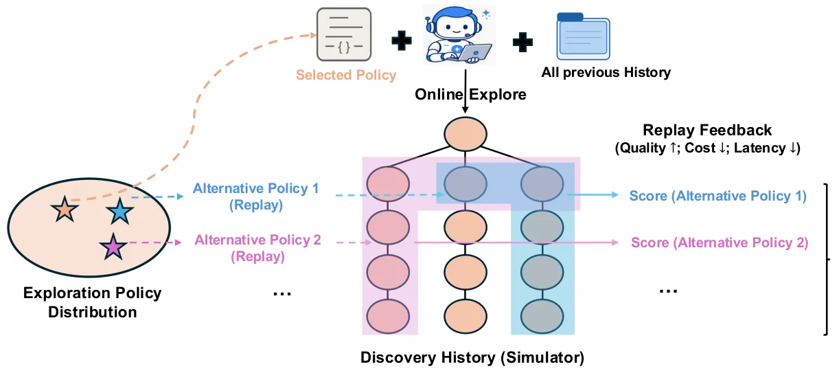
Figure 2: Discovery history as a replay simulator. A deployed policy explores online and produces a structured discovery tree with full observations at each node. Thousands of candidate policies can then be tested inside this simulator by choosing alternative branches, orders, concurrency levels, and stopping rules. Since all outcomes are pre-stored, a single costly online run enables thousands of rapid, zero-execution-cost off-policy evaluations.

Method

1. Online rollout: policy frozen, history growing

Outer iterations are indexed by $t=1,2,\ldots$, starting from an initial policy $\pi_1$ and empty history $\mathcal{H}_0=()$. At iteration $t$, policy $\pi_t$ guides a new online rollout with access to the completed discovery history $\mathcal{H}_{t-1}$. That history supplies context for exploration but stays separate from the new tree being constructed, and the policy code remains fixed throughout the rollout. Let $\mathcal{T}_t^{k}$ be the new discovery tree after $k$ completed decision rounds, with $\mathcal{T}_t^{0}=\{r\}$, and let the rollout allow at most $K_1$ rounds.

At round $k\leq K_1$, the exploration policy chooses a batch $C_t^{k}\in A(\mathcal{T}_t^{k};W)$ and each node $v\in C_t^k$ is assigned to a worker. The discovery agent uses $v$'s saved workspace and available context to produce a new candidate, and the evaluator assesses the result. These attempts run in parallel and each produces one new child of its selected parent; attaching the completed children yields $\mathcal{T}_t^{k+1}$ while all previously recorded nodes remain unchanged. This transition is stochastic, because the discovery agent may generate different outcomes from the same starting workspace. In the next round, the newly created child becomes the selectable leaf of an extended branch while the root remains selectable for opening further branches. The rollout ends when the policy selects an empty batch or completes $K_1$ rounds; the final tree is recorded as $\mathcal{T}_t$ and appended to history:

$$\mathcal{H}_t=\mathcal{H}_{t-1}\cup\{\mathcal{T}_t\}$$

2. Offline replay: a deterministic Child operator

During the offline phase of outer iteration $t$, the history $\mathcal{H}_t$ stays fixed while the method constructs and evaluates $M\geq 1$ policy versions $\pi_t^{0},\ldots,\pi_t^{M-1}$, starting from $\pi_t^{0}=\pi_t$. Each version is evaluated separately on every historical tree $\mathcal{T}_i$, $i=1,\ldots,t$, before the next version is developed from the resulting feedback. Notation: $m$ indexes policy versions, $i$ indexes replay worlds, and $k$ counts decision rounds within one policy–world evaluation.

For each pair $(m,i)$, replay resets the policy's per-rollout state and starts from $\mathcal{T}_i^{m,0}=\{r\}$, where $\mathcal{T}_i^{m,k}\subseteq\mathcal{T}_i$ is the subtree revealed after $k$ completed rounds. The full recorded tree $\mathcal{T}_i$ never changes; only the portion observed by the policy evolves. At each decision, $\pi_t^{m}$ selects a batch $C_i^{m,k}\in A(\mathcal{T}_i^{m,k};W)$ from the revealed observations. Unlike online execution, replay returns recorded children of the selected nodes deterministically instead of generating new candidates:

$$\mathcal{T}_i^{m,k+1}=\mathcal{T}_i^{m,k}\cup\bigcup_{v\in C_i^{m,k}}\operatorname{Child}(v;\mathcal{T}_i,\mathcal{T}_i^{m,k})$$

The $\operatorname{Child}$ rule is what makes the whole mechanism work. For $v\neq r$, it returns $v$'s unique recorded child on $\mathcal{T}_i$ if one exists; since $v$ is a leaf of $\mathcal{T}_i^{m,k}$, that child is necessarily still unrevealed. For $v=r$, it returns the earliest-created child of $r$ outside $\mathcal{T}_i^{m,k}$, thereby opening one previously unrevealed branch. In either case $\operatorname{Child}(v;\mathcal{T}_i,\mathcal{T}_i^{m,k})=\emptyset$ when no recorded continuation remains. Newly revealed nodes expose their stored observations before the policy makes its next decision. Replay allows at most $K_2$ decision rounds (each nonempty batch counts as one) and terminates when the policy selects $C_i^{m,k}=\emptyset$, when $k=K_2$ is reached, or when $\mathcal{T}_i^{m,k}=\mathcal{T}_i$, meaning all recorded nodes have been revealed. The number of completed rounds at termination is $k_i^{m,\star}\in\{0,\ldots,K_2\}$, giving the final subtree $\mathcal{T}_i^{m,k_i^{m,\star}}\subseteq\mathcal{T}_i$.

Replay therefore evaluates how far to pursue each opened branch, how to group attempts into parallel batches, and when to open another branch or stop. Those decisions may differ across policies, but each branch is traversed in its recorded parent–child order and no outcomes beyond $\mathcal{T}_i$ are ever generated.

3. The replay objective: quality, cost, parallelism

Let $N_i^{m}=|\mathcal{T}_i^{m,k_i^{m,\star}}|-1$ be the number of revealed non-root nodes. Replay itself executes no new discovery attempts, yet $N_i^{m}$ counts the generation–evaluation requests that the trajectory represents. For fixed coefficients $\beta_1,\beta_2\geq 0$, the replay score is

$$V_i^{m}=\underbrace{\max_{v\in\mathcal{T}_i^{m,k_i^{m,\star}}} s_v}_{\text{discovery quality}}-\underbrace{\beta_1 N_i^{m}}_{\text{execution cost}}+\underbrace{\beta_2\frac{N_i^{m}}{\max\{1,k_i^{m,\star}\}}}_{\text{parallelism bonus}}$$

The first term is the best solution quality attained during replay, the second penalizes the number of attempted generations, and the third (for a nonempty replay) rewards the average number of attempts executed per decision round, favoring policies that batch useful continuations instead of executing them sequentially. This is also why the replay score is not a trivial re-read of the historical best: on the very same tree, a policy can score lower by revealing less or by batching worse.

4. Policy improvement and selection, with a bounded monotonicity guarantee

The score of policy version $\pi_t^{m}$ is its average replay score across the fixed history:

$$V^{m}=\frac{1}{t}\sum_{i=1}^{t}V_i^{m}$$

The offline phase begins by evaluating the current policy $\pi_t^{0}=\pi_t$. For each $m=0,\ldots,M-1$, a fixed LLM-based policy-development agent examines the replay trajectories and scores of $\pi_t^{m}$ together with feedback from earlier revisions, identifies successful decisions and recurring failures, then revises the executable policy code to produce $\pi_t^{m+1}$, which is evaluated on the same $t$ replay worlds. Replay feedback is available to the development agent between revisions.

After $M$ revisions, the next online policy is selected from all evaluated versions: $\pi_{t+1}=\pi_t^{m^{\star}}$ with

$$m^{\star}\in\operatorname*{arg\,max}_{m\in\{0,\ldots,M-1\}}V^{m}$$

Because the candidate set includes the current policy, this selection satisfies $V^{m^{\star}}\geq V^{0}$: on the fixed history $\mathcal{H}_t$, the selected policy is no worse than the current one in average replay score. It is then deployed online to collect $\mathcal{T}_{t+1}$, expanding the history available for the next offline improvement phase. Only the exploration-policy code changes across the whole loop; the underlying models, evaluator, and execution interfaces remain fixed.

flowchart TD
  P0["initial exploration policy pi_1 refine W workspaces in parallel"] --> ON["online rollout at most K1 rounds policy code frozen"]
  ON --> AG["discovery agent resumes parent workspace proposes new candidate"]
  AG --> EV["evaluator scores s_v stores snapshot and diagnostics"]
  EV --> TREE["attach children to obtain discovery tree T_t"]
  TREE --> HIST["append to history H_t = H_t-1 union T_t"]
  HIST --> SIM["historical tree pool becomes replay simulator all outcomes recorded"]
  SIM --> REP["replay at most K2 rounds Child operator reveals recorded children"]
  REP --> SCORE["score V_i^m quality minus cost plus parallelism bonus"]
  SCORE --> DEV["policy development agent reads traces and scores rewrites policy code"]
  DEV --> MORE{"M versions evaluated"}
  MORE -->|no feedback visible| REP
  MORE -->|yes| SEL["pick argmax V^m as pi_t+1 no worse than V^0"]
  SEL -->|redeploy| ON
  SEL --> OUT["collect T_t+1 online simulator pool grows"]
  OUT --> ON

Diagram: the meta-level loop. The left half is online (policy frozen, tree growing, history accumulating); the right half is offline (the same historical trees are replayed, scored, and used to rewrite $M$ policy versions). The two halves are joined by the $\operatorname{Child}$ operator and the argmax selection over $V^m$.

5. What the orchestration layer actually looks like in code

Appendix B pins the abstraction to a concrete programming interface and, in doing so, exposes the engineering limits of the method. The online exploration prompt requires the discovery agent to inspect the complete available discovery history before proposing a new solution, to reason explicitly about both successful and failed attempts, and to avoid repeatedly exploiting a locally saturated direction.

The replay-side policy-improvement prompt is stricter: the agent may edit only one file {method_file} and implement OptimalPolicy.solve(self, question, budget=None); it is explicitly forbidden from solving the scientific task itself or editing any other program. The environment is described as a frozen, irregular branch × attempt grid in which a policy either opens a root or refines the next cell of an already-open branch, each revealed cell costing one probe. The policy sees only the cells it has revealed so far; unrevealed scores are unknown. The evaluator sweeps the policy's single beta knob and ranks the resulting curve by

pareto.reward = pareto.auc - lambda * parallel_penalty

where pareto.auc rewards reaching high per-trace attainment with few total probes, and parallel_penalty is the mean of effective_sequential_rounds / total_probes over the sweep — the prompt-level twin of the parallelism bonus in Equation (1). A second hook, plan_grid(context) -> GridPlan, runs before a new live grid is created: it makes no within-episode decision, must never inspect a current episode's outcomes, and must always return a non-None GridPlan(branch_count=W, refine_count=R), including an explicit conservative bootstrap plan with a factual reason when history is empty. W and R are arbitrary integers rather than fixed presets, subject to 0 <= R <= context.hard_max_refine_count. The most consequential sentence is this one: in replay, a requested plan beyond the frozen trace's context.trace_branch_count or context.trace_refine_count is out of support and cannot earn replay reward. That is the interface-level expression of the fact that replay can only reveal recorded outcomes.

Experiments

All three domains share one controlled design. Dream-RSI and the primary baseline, Recursive Fixed Exploration, use the same discovery agent, evaluator, initialization, and resource constraints, and both start from the same manually designed exploration policy — a simple parallel-refinement strategy that launches multiple independent exploration workspaces, each maintaining its own local discovery trajectory and repeatedly refining its current candidate using the history accumulated inside that workspace. Round 1 is therefore identical for both methods. From round 2 onward, fixed exploration keeps its policy static while Dream-RSI rewrites and redeploys the policy each round by dreaming over accumulated global history. Discovery cost is the cumulative number of discovery-agent calls. Agents are driven through the Gemini CLI with Gemini-3.1 Pro and Gemini-3.7-Flash: per round, fixed exploration runs 10 parallel workspaces × up to 11 refinement steps = 110 calls on Pro and 32 × 20 = 640 calls on Flash. Dream-RSI keeps identical per-round budgets, running 5 recursive rounds on Lasso and 10 on the mathematics tasks.

Algorithm engineering: the Lasso regularization path

Task definition (Appendix A): given a feature matrix $X\in\mathbb{R}^{n\times p}$, response $y\in\mathbb{R}^{n}$, and a decreasing sequence $\lambda_1>\cdots>\lambda_K$,

$$F_k(w):=\frac{1}{2n}\|y-Xw\|_2^2+\lambda_k\|w\|_1,\qquad w_k^{\star}\in\arg\min_{w\in\mathbb{R}^{p}}F_k(w)$$

A candidate solver returns approximate coefficients $\widetilde{W}=(\widetilde w_1,\ldots,\widetilde w_K)$ and passes the benchmark's objective-value check only if

$$F_k(\widetilde w_k)\leq F_k(w_{k,\mathrm{sklearn}})+10^{-6}\quad\text{for every }k$$

with correctness checked on fresh instances distinct from the timing instances; if any required check fails, the search score is zero. Otherwise, letting $\mathcal{I}$ denote the timing instances and $t_i$ the time to compute the complete regularization path on instance $i$, the search score is the inverse geometric-mean runtime:

$$R_{\mathrm{search}}=\Big(\prod_{i\in\mathcal{I}}t_i\Big)^{-1/|\mathcal{I}|}$$

The setup follows SimpleTES with the same 17 synthetic instances covering diverse dimensionality, sparsity, feature correlation, and active-set structure. To test whether discovered algorithms generalize beyond the search distribution, they are additionally evaluated on six held-out downstream datasets spanning biological and non-biological domains. The table below reports runtime in milliseconds (lower is better).

Method	Discovery agent	Calls	Gisette	RCV1	DNA	Leukemia	Colon	Duke Breast	Avg.
sklearn	—	—	11275.2	252881.7	93.8	227.2	229.8	374.0	44180.3
glmnet	—	—	9063.6	73072.8	351.9	45.0	24.2	47.7	13767.5
SimpleTES	gpt-oss-120b	51,200	3141.9	19625.6	15.9	15.5	11.6	18.1	3804.8
SimpleTES †	gpt-oss-120b	51,200	8651.0	41143.1	37.6	28.2	19.5	31.1	8318.4
Recursive Fixed Exploration	Gemini-3.1-Pro	550	1861.8	19550.1	41.5	26.1	14.5	28.4	3587.1
Recursive Fixed Exploration	Gemini-3.7-Flash	3200	1133.1	13873.0	29.8	24.1	15.7	24.4	2516.7
Dream-RSI	Gemini-3.1-Pro	317	2841.0	14616.0	49.9	30.2	16.4	32.5	2931.0
Dream-RSI	Gemini-3.7-Flash	1879	1091.9	12923.4	31.4	21.0	12.2	23.6	2350.6

Table 1: Lasso-path solver runtime (ms, lower is better) on six held-out datasets, with discovery cost measured as cumulative discovery-agent calls. Numbers from Figure 3(a) of the paper.

Two things matter when reading this table. First, Dream-RSI obtains a better quality–compute trade-off on both backbones: with Pro it cuts the average runtime across the six held-out datasets from 3587.1 ms to 2931.0 ms while using 317 discovery-agent calls instead of 550 (about 1.7×), and with Flash it goes from 2516.7 ms to 2350.6 ms using 1879 calls instead of 3200. It is not buying quality with more compute; it spends less and lands better. Second, against SimpleTES — which uses 51,200 generations — Dream-RSI achieves a lower average downstream runtime with roughly two orders of magnitude fewer discovery-agent calls (162× as stated in the abstract).

The table also contains cells that go against Dream-RSI. On the smaller datasets Gisette, DNA, Leukemia, Colon, and Duke Breast, the Pro variant (2841.0 / 49.9 / 30.2 / 16.4 / 32.5) is slower than fixed exploration (1861.8 / 41.5 / 26.1 / 14.5 / 28.4); its average advantage is carried mainly by the large-scale RCV1 column (14616.0 versus 19550.1, the lowest in that column). The paper's reading is that the two backbones discovered programs with different temperaments: the Pro program is particularly well suited to large matrices such as RCV1, while the Flash program is more general-purpose and consistent across problem scales — the Flash variant is lowest in 5 of the 6 datasets.

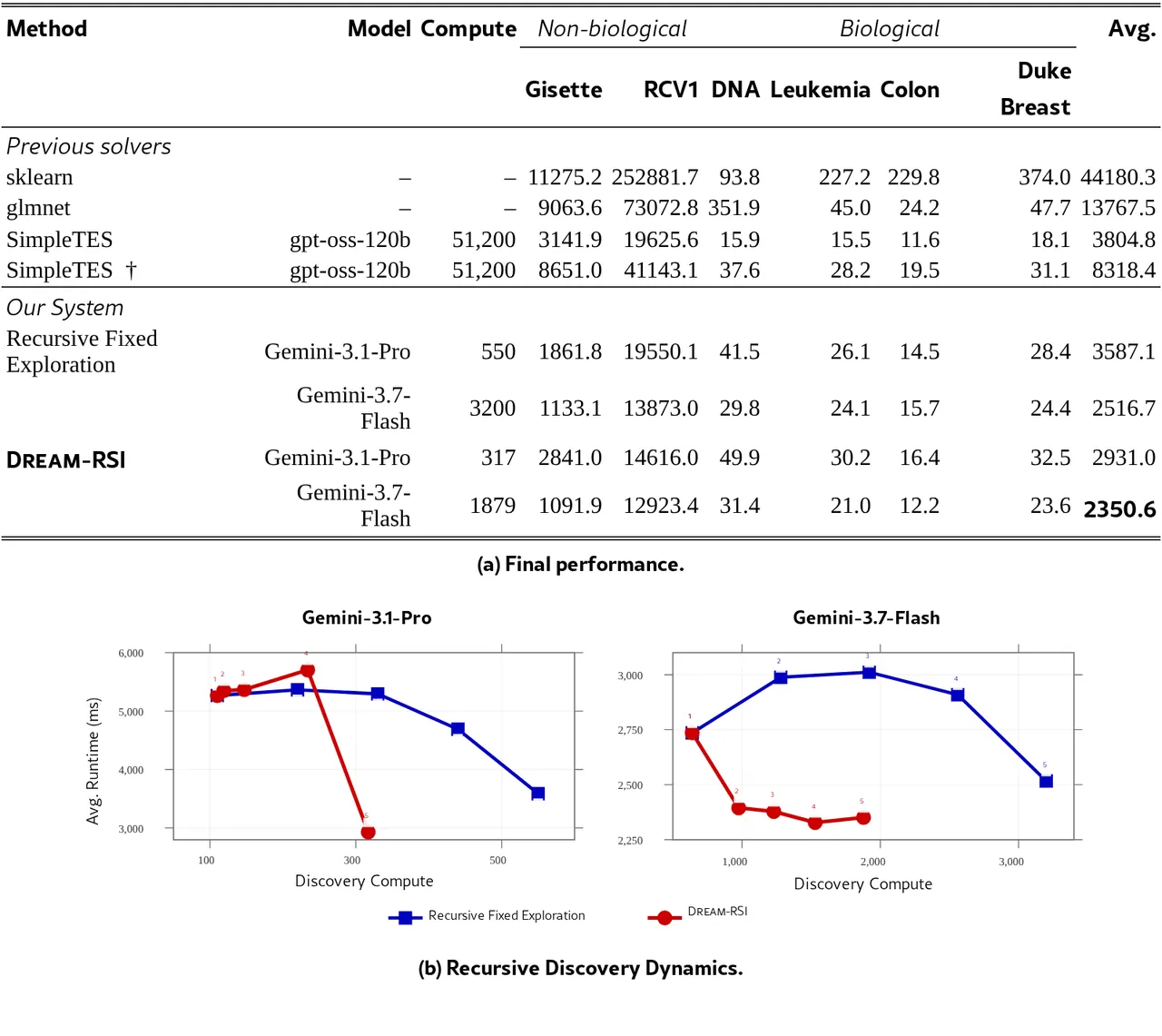
Figure 3: (a) final performance on Lasso-path discovery; (b) recursive discovery dynamics — downstream performance against cumulative discovery compute. The two methods coincide in round 1 by design; afterwards fixed exploration keeps a static policy while Dream-RSI refines and redeploys its policy each round, so the trajectories diverge markedly on both Gemini-3.1-Pro and Gemini-3.7-Flash.

What the discovered solver actually does

This is one of the most convincing pieces of evidence in the paper, because it shows that improving the exploration policy buys a structurally different algorithm rather than better hyperparameters for the same one. Unlike SimpleTES, which switches between LARS and coordinate descent according to problem dimensions, the discovered solver places adaptivity inside the active-set optimization itself: strong-rule screening combined with Cauchy–Schwarz-based KKT pruning, recomputing exact gradients selectively only when the bound cannot certify a feature, and falling back to a full refresh when pruning becomes ineffective. This adaptive verification scheme is integrated with efficient active-set bookkeeping (disjoint lists with O(1) swap-delete), lazy Gram-matrix construction, and hardware-aware implementation.

// Appendix C, Listing 3: Lasso-path solver discovered by Dream-RSI (excerpt)
// Branch-free soft-thresholding via std::abs and std::copysign
static inline double soft_thresh(double z, double gamma) {
  double abs_z = std::abs(z);
  double val = abs_z - gamma;
  return std::copysign(val > 0.0 ? val : 0.0, z);
}

// Dual-Phase Adaptive Cauchy-Schwarz KKT Pruning
double d2 = 0.0;
const double* RESTRICT r_curr_ptr = ASSUME_ALIGNED(r_padded, 64);
const double* RESTRICT r_ref_ptr  = ASSUME_ALIGNED(r_ref_padded, 64);
#pragma omp simd reduction(+:d2) aligned(r_curr_ptr, r_ref_ptr: 64)
for (int k = 0; k < n_padded; ++k) {
  double diff = r_curr_ptr[k] - r_ref_ptr[k];
  d2 += diff * diff;
}

The two snippets correspond to two techniques described in the text: soft-thresholding is made branch-free to avoid mispredictions inside the coordinate-descent inner loop, and the Cauchy–Schwarz pruning first builds a vectorizable bound from the squared difference $d_2$ between current and reference residuals, computing an exact gradient only when the bound is inconclusive. Inner-product loops throughout use 4-way register blocking (sum0..sum3) with 64-byte alignment. None of this was specified in a human-written prompt; it emerged through repeated policy rewrites driven by replay feedback.

Mathematics optimization: three tasks at a 50× budget gap

The three tasks span discrete combinatorial optimization, geometric optimization, and functional optimization. The sum–difference problem asks for a finite set $A\subset\mathbb{Z}$ whose normalized sumset is large relative to its normalized difference set:

$$\Gamma(A):=\frac{\log\!\left(|A+A|/|A|\right)}{\log\!\left(|A-A|/|A|\right)},\quad A+A:=\{a+a':a,a'\in A\},\ A-A:=\{a-a':a,a'\in A\}$$

Circle packing in a unit square ($n\in\{26,32\}$) asks for centers $(x_i,y_i)\in[0,1]^2$ and radii $r_i\geq 0$ satisfying $r_i\leq x_i\leq 1-r_i$, $r_i\leq y_i\leq 1-r_i$, and non-overlap $(x_i-x_j)^2+(y_i-y_j)^2\geq(r_i+r_j)^2$, maximizing $\sum_i r_i$. The autocorrelation inequality task minimizes the peak of the autoconvolution, $\Phi_1(f):=\max_{t\in[-1/2,\,1/2]}(f*f)(t)$ with $(f*f)(t):=\int_{\mathbb{R}}f(t-x)f(x)\,dx$, over non-negative integrable $f$ supported on $[-1/4,1/4]$ with $\int_{-1/4}^{1/4}f(x)\,dx=1$.

Method	LLM	Sum Diff (higher is better)	Auto Correlation (lower is better)	Circle Packing (higher is better)
AlphaEvolve	Gemini-2.0 Pro + Flash	—	1.455700	2.635862
AlphaEvolveV2	Gemini-2.0 Pro + Flash	1.121936	—	2.635983
OpenEvolve	—	—	1.460000	—
CodeEvolve	—	—	—	2.635980
ShinkaEvolve	Mixed	—	1.457800	2.635982
TTS-Discovery	Qwen3-8B	—	—	2.635983
ThetaEvolve	Distilled-Qwen3-8B	—	1.493000	2.635983
EvoX	Gemini-3.0-Pro	—	1.458900	2.635900
SimpleTES	GPT-OSS-120B	1.143975	1.453675	2.635983
Recursive Fixed Exploration	Gemini-3.1-Pro	1.144047	1.456001	2.635983
Dream-RSI	Gemini-3.1-Pro	1.145427	1.456375	2.635983

Table 2: Mathematical discovery tasks (Table 1 of the paper). Dream-RSI and fixed exploration both use Gemini-3.1 Pro over 10 recursive rounds.

On sum–difference, Dream-RSI reaches 1.145427, ahead of fixed exploration's 1.144047 and SimpleTES's 1.143975. On circle packing it reaches 2.635983, matching the strongest reported result among the compared systems (AlphaEvolveV2, TTS-Discovery, ThetaEvolve, and SimpleTES all report the same value). The autocorrelation column should be read honestly: lower is better there, and Dream-RSI's 1.456375 is slightly worse than fixed exploration's 1.456001 and clearly worse than SimpleTES's 1.453675 — the paper describes this as "remaining competitive". The real gap is budget: SimpleTES needs 51,200 generations where Dream-RSI uses fewer than 1,000. In this domain, the defensible claim is parity at roughly 1/50 of the budget, not superiority.

GPU kernel engineering: four KernelBench tasks

Kernel engineering requires reasoning jointly about algorithmic structure, memory access, parallelization, and hardware-specific optimizations, which makes it a substantially different testbed for cross-domain generalization. The tasks are VGG16, LayerNorm, ConvDiv, and ConvMax from KernelBench; candidates are scored by execution performance measured as inverse runtime (1/ms) subject to correctness checks against the reference implementation. Gemini-3.1 Pro is the coding agent, and the comparison against fixed exploration uses the same evaluation protocol and initialization.

KernelBench task	Dream-RSI vs. fixed exploration	Comparison basis
VGG16	2.43× fewer generations	comparable final performance
LayerNorm	1.79× fewer generations	comparable final performance
ConvDiv	2.09× higher score	similar discovery budget
ConvMax	1.44× higher score	similar discovery budget

Table 3: GPU kernel engineering results (Figure 4 of the paper). Higher is better on all four tasks; performance is measured in 1/ms.

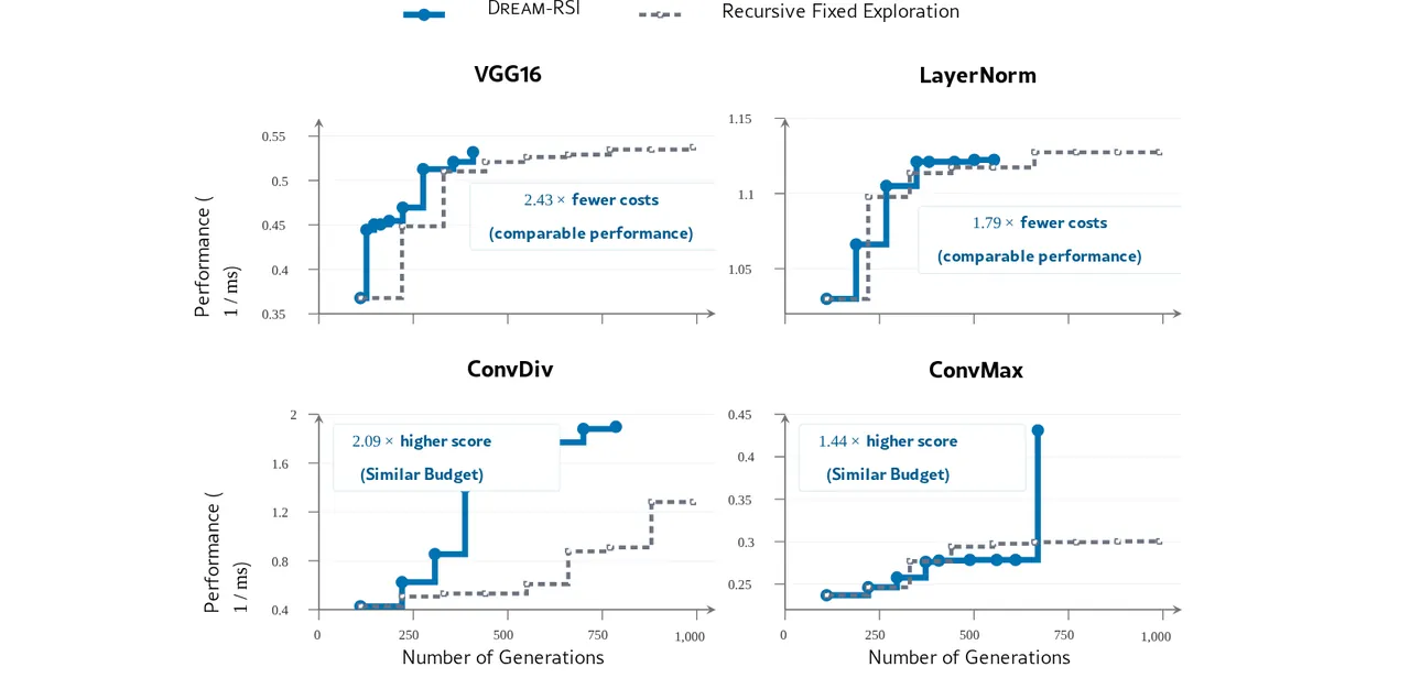
Figure 4: GPU kernel engineering. Discovery performance as a function of the number of generations. On VGG16 and LayerNorm, Dream-RSI reaches comparable performance with 2.43× and 1.79× fewer generations; on ConvDiv and ConvMax it achieves 2.09× and 1.44× higher performance under comparable budgets.

Two analyses: semantic guidance hurts, exploration effort adapts

The first analysis challenges the common practice of summarizing history into advice and feeding it back into the prompt. The authors build the natural alternative — abstract prior trajectories into high-level directional insights and inject them as explicit semantic guidance in subsequent rounds — and apply it to both fixed exploration and Dream-RSI. Under equivalent discovery budgets, the guided variants consistently underperform their unguided counterparts in both paradigms. The proposed explanation is that in long-horizon discovery, where multiple parallel threads are deployed, imposing strong semantic inductive biases about future search directions over-constrains the search space and impedes diverse exploration.

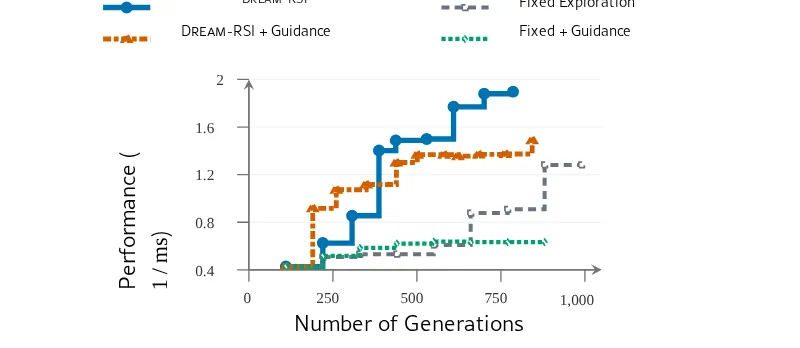
Figure 5: Discovery performance on ConvDiv. Using history as an interactive replay simulator outperforms using it only as guidance.

The second analysis looks at how the learned policy's behavior changes over rounds. On ConvDiv, round-best performance rises monotonically from E0 to E8 while the number of evaluated attempts per round follows a clearly adaptive shape: effort is first cut from 110 attempts to 50 while performance climbs quickly (saving compute), then raised back to roughly 90 once progress plateaus, coinciding with further gains. In other words, the cost and parallelism terms of the replay objective really do write "when to save" and "when to fan out" into the policy code, rather than merely pushing the score up.

Recursive round	E0	E1	E2	E3	E4	E5	E6	E7	E8
Round-best performance (1/ms)	0.427	0.625	0.855	1.403	1.488	1.499	1.770	1.880	1.898

Table 4: Round-best performance on ConvDiv across recursive execution rounds (Figure 6(a) of the paper). Figure 6(b) shows evaluated attempts per round dropping from 110 to 50 and rising back to about 90 once progress plateaus.

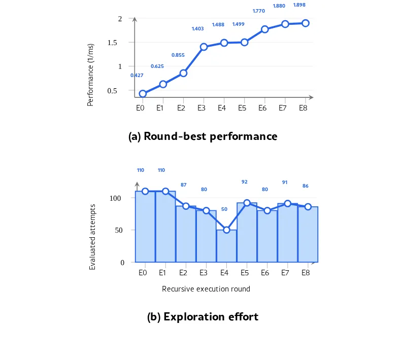
Figure 6: Evolution of exploration behavior on ConvDiv. (a) Round-best performance across recursive execution rounds. (b) Number of evaluated attempts in each round — the policy first conserves compute, then increases exploration effort again when progress stalls.

Limitations

1. Replay can only reveal recorded outcomes, so genuinely novel directions cannot be scored. This is a constraint the authors state at the prompt level: a requested plan beyond the frozen trace's trace_branch_count or trace_refine_count is out of support and earns no replay reward. The world model is therefore valid only over the realized search space — it can reorder branches, regroup parallel attempts, and reset stopping points, but it cannot assign a score to a direction that was never tried. Coverage of the history pool sets the ceiling on dreaming, which is the same class of risk as model bias in model-based RL, where a policy exploits holes in the learned model.

2. The monotonicity guarantee is narrower than the framing suggests. $V^{m^{\star}}\geq V^{0}$ holds only in average replay score on the fixed history $\mathcal{H}_t$; it does not imply that the next online round performs better. The paper reports no correlation measure, confidence interval, or theoretical bound linking replay score to online gain, and the selection pressure may favor policies that are good at harvesting old trees rather than at opening productive new branches.

3. Quality gains in mathematics are thin, and autocorrelation actually regresses. Dream-RSI's 1.456375 is worse than fixed exploration's 1.456001 on a lower-is-better metric, circle packing ties several systems at 2.635983, and the sum–difference lead appears in the fourth decimal place. The defensible advantage is budget (fewer than 1,000 generations versus 51,200), not solution quality.

4. The key ablation covers a single task, and hyperparameters are not reported. The negative result on semantic guidance is shown as one curve pair on ConvDiv, with no cross-task or cross-budget statistics. $\beta_1$, $\beta_2$, $M$, $K_1$, and $K_2$ appear only symbolically in the text; concrete values and the range of the beta sweep are not tabulated. With the repository code not yet released, third-party reproduction currently depends on the prompts and source in Appendices B and C.

5. The evaluation surface is narrow. Discovery agents are limited to two Gemini models, and the tasks are confined to three domains with automatically checkable objectives. The paper has no dedicated limitations section, so these boundaries have to be read out of the main text and appendices. Settings where evaluation itself is not repeatable — for example physical robot experiments — are not addressed, and that is exactly where a replay simulator built from recorded outcomes would be hardest to justify.

Takeaways and Outlook

Dream-RSI's contribution is not a new architecture but a change in the status of "history": from context into environment. Three transferable conclusions stand out. First, the cost of meta-level optimization is dominated by feedback latency rather than raw compute — find a recorded stand-in for the feedback and the loop can speed up by one to two orders of magnitude. Second, "executable policy code plus a frozen decision interface" is the minimal structure that lets an LLM rewrite its own orchestration layer without losing control; OptimalPolicy.solve and GridPlan are the concrete shape of that interface here. Third, structured experience replay can beat semantic experience summarization, which runs against the widespread engineering instinct of stuffing summarized history back into the prompt.

For robotics and embodied AI, there is a direct analogue. Real-robot data is expensive, and an executed skill tree — successful trajectories, failure diagnostics, and cost records — is already a replay world. One can re-plan offline over which branch to try first, how many to fan out, and when to stop, without touching the hardware again, with digital-twin and simulation assets serving as additional ways to grow the history pool. The boundary still applies: a replay world covers only realized actions and states, so any direction that needs new physical interaction to validate must still go online. What Dream-RSI removes is trial-and-error cost at the orchestration layer, not the cost of exploration itself.

Golden Quote

A single expensive online discovery run can support many inexpensive evaluations of alternative exploration strategies — because all execution outcomes are already stored in the tree, evaluating a new policy only requires reading past records, not rerunning the discovery agent.

This analysis is based on the full text of arXiv:2609.14858v1, including Appendix A (task definitions), Appendix B (prompts), and Appendix C (discovered programs). Source: https://arxiv.org/abs/2609.14858.