Juno: Taming Predictive Latents for Vision-Language-Action Models

Paper Metadata

Title: Juno: Taming Predictive Latents for Vision-Language-Action Models

Authors: Yuchen Zhu, Chenyi Xu, Yulin Zhang, Gang Xu, Wentao Zhu (University of Science and Technology of China; Eastern Institute of Technology, Ningbo; Hangzhou Dianzi University; ShanghaiTech University)

Links: arXiv:2610.09940 (v2, 2026-10-11) · project page · code repository · Hugging Face model entry LightningNO1/Juno

Code status: The repository releases the full training stack for the Bridge/Fractal policy-learning stage: the juno-policy model (JEPA interface, patch fusion, MoT reasoning branch), LeRobot data mixtures and transforms, trainer, and launcher, under an MIT license derived from StarVLA with attribution clauses preserved. The README TODO list still leaves JEPA pretraining code, TTT code, and checkpoint release unchecked, and docs/reproducibility.md states plainly that the public launcher covers only the policy stage and that README scores are reported paper results, not runs of this repository. Reproduction attempts should treat configs/bridge_fractal_jepa7_mot_1005.yaml as the authoritative recipe.

Background and Motivation

Predictive latents are naturally attractive for vision-language-action (VLA) models. Joint-embedding predictive architectures (JEPAs) predict masked or future observations in representation space instead of reconstructing pixels, so the states they learn carry implicit information about what happens next. The authors argue, however, that making such latents useful across the three phases of a VLA system - pretraining, policy learning, and deployment - runs into three distinct failures. The first is mismatch with embodiment-specific control: encoders pretrained on generic video, such as V-JEPA 2, respond sluggishly to local robot-object interaction. In Figure 2(a) their patch-wise temporal cosine distance maps are nearly uniform, while LeWM's patch maps light up precisely over the manipulation region; in Figure 2(b) even LeWM's CLS state stays almost flat during the pick-and-place phase of an episode, showing how a global token can be diluted by static background and appearance. The second failure is interference with action learning: bolting future prediction onto the VLA backbone perturbs the very representations used for action generation. The ablation gives direct evidence - removing patch fusion while keeping the predictive branch drops average success to 53.9%, below the 60.9% of a model with no Juno components at all. The third failure is teacher miscalibration under distribution shift: under strong observation noise or abrupt illumination change, a frozen JEPA teacher becomes unreliable itself, and the policy coupled to it collapses.

Prior work addresses one corner each. VLA-JEPA-style methods attach JEPA features to a VLA but keep the pathway between prediction and action generation shallow or serial; test-time methods such as WAM-ttt, TTT-VLA, and VANE adjust latents or prompts at deployment, but most trust only successful rollouts or treat the world model as a fixed scorer. Juno's answer is one model in three roles: the same action-conditioned JEPA is first pretrained on embodiment-matched trajectories with a control-aligned objective, then frozen as a teacher that distills future states during policy learning, and finally unfrozen at deployment as a fully adaptable dynamics model that absorbs every interaction, failures included.

Preliminaries

Action-conditioned JEPA world model (LeWM). A JEPA encodes an observation into a latent state and predicts the latent state of a future observation rather than decoding pixels. LeWM is the lightweight control-oriented instantiation: trained end to end from pixels with roughly 15M parameters in its ViT-Tiny configuration, its predictor conditions on the current CLS state and the executed action. Juno inherits its interface: the encoder emits a CLS token and a patch-token grid, and the predictor emits the predicted next-frame CLS.

VLA policy with a flow-matching action head. The policy maps an observation and a language instruction (plus proprioception when available) to an action distribution. Juno instantiates this as a Qwen3-VL-4B-Instruct backbone with a GR00T-style flow-matching DiT action decoder; actions are predicted as 16-step chunks, trained with eight noise/time samples per chunk and inferred with four Euler steps.

Mixture-of-Transformers (MoT). The vision-language branch and the predictive reasoning branch hold separate non-embedding parameters (attention projections, MLPs, layer norms) while sharing a single causal attention graph: the two branches see each other at every layer but transform their own tokens with their own weights. This lets future prediction own a dedicated parameter set without contaminating the representations used for action generation.

Method

The interface of one action-conditioned JEPA

Write a robot trajectory as $\tau=\{(o_t,a_t,o_{t+1})\}_{t=1}^{T}$ with encoder $f_\theta$ and latent predictor $g_\phi$:

$$[c_t,P_t]=f_\theta(o_t),\qquad \hat{c}_{t+1}=g_\phi(c_t,a_t),\qquad \mathcal{L}_{\mathrm{JEPA}}=\mathcal{L}_{\mathrm{pred}}(\hat{c}_{t+1},c_{t+1})+\lambda_{\mathrm{reg}}\mathcal{R}(c), \tag{1}$$

where $c_t\in\mathbb{R}^D$ is the CLS token, $P_t=[p_{t,1},\ldots,p_{t,M}]\in\mathbb{R}^{M\times D}$ is the patch-token grid, and $\mathcal{R}$ is the latent regularizer (implemented as SIGReg with weight 0.2, 1024 projections, and 17 knots). The prediction $\hat{c}_{t+1}$ is computed from $(c_t,a_t)$ while the target $c_{t+1}$ is encoded from the observed next frame; this action-conditioned structure is precisely what allows the same objective to be reused later for test-time adaptation. LeWM keeps only $c_t$ as the state for planning and discards $P_t$ for efficiency, yet Figure 2(b) shows the CLS token barely moving during pick-and-place: sparse object or contact changes are diluted by static background. Juno's first intervention targets exactly this bottleneck.

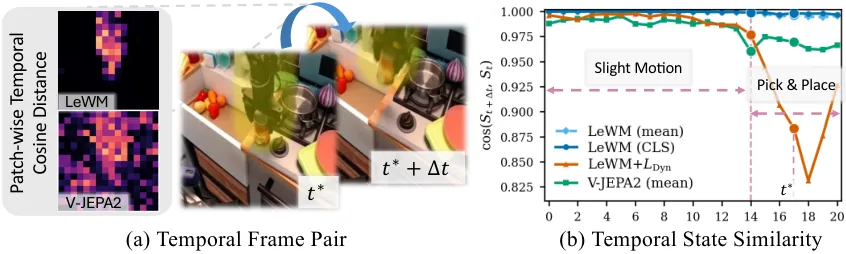
Figure 1: motivating evidence (paper Fig. 2). (a) Patch-wise temporal cosine distance between frames t* and t*+dt: LeWM responds locally over the manipulation region while V-JEPA2 is nearly uniform. (b) Temporal state similarity cos(c_t, c_{t+dt}) across an episode: LeWM (CLS) stays almost flat between the slight-motion segment (t at most 14) and the pick-and-place segment (t above 14), whereas LeWM trained with the Dynamic CLS loss becomes sensitive during pick-and-place; mean-pooled baselines are shown for reference.

Control-aligned pretraining: the Dynamic CLS loss

The idea is to supervise the CLS token with patch-level change, in two stages. Stage one trains LeWM with the standard objective of Eq. 1, by which point patch tokens already respond reliably to local interaction. Stage two freezes that encoder as a patch supervisor $\bar{f}$, writing $[\bar{c}_t,\bar{P}_t]=\bar{f}(o_t)$, and continues training the trainable encoder against targets that cannot drift - the frozen supervisor is a stop-gradient reference. For each sampled transition, the change of the i-th frozen patch token and its magnitude are

$$\Delta\bar{p}_{t,i}=\bar{p}_{t+1,i}-\bar{p}_{t,i},\qquad m_{t,i}=\frac{\lVert\Delta\bar{p}_{t,i}\rVert_2}{\sqrt{D}}. \tag{2}$$

A motion-aware aggregation then converts relative patch-change magnitudes into soft weights:

$$\widetilde{m}_{t,i}=\frac{m_{t,i}}{\max\!\left(M^{-1}\sum_{j=1}^{M}m_{t,j},\,\epsilon\right)},\qquad \alpha_{t,i}=\frac{\exp(\widetilde{m}_{t,i}/\tau)}{\sum_{j=1}^{M}\exp(\widetilde{m}_{t,j}/\tau)}, \tag{3}$$

where $\tau$ is a temperature (0.5 in the implementation), $\epsilon$ prevents division by zero, and $M$ is the patch count. The motion-weighted patch target is $u_t=\sum_{i=1}^{M}\alpha_{t,i}\Delta\bar{p}_{t,i}$, the trainable encoder's CLS transition is $\Delta c_t=c_{t+1}-c_t$, and the auxiliary loss is

$$\mathcal{L}_{\mathrm{dyn}}(\theta)=\mathbb{E}_{(o_t,a_t,o_{t+1})\sim\mathcal{D}}\left[\lVert\Delta c_t-u_t\rVert_2^2\right]. \tag{4}$$

Note that $a_t$ does not enter this auxiliary target directly; it remains part of the action-conditioned JEPA objective of Eq. 1. The second-stage objective is

$$\mathcal{L}_{\mathrm{LeWM+Dyn}}=\mathcal{L}_{\mathrm{JEPA}}+\lambda_{\mathrm{dyn}}\mathcal{L}_{\mathrm{dyn}}. \tag{5}$$

The effect is to keep LeWM's single-CLS interface, so downstream consumers still see one compact state, while making $c_t$ responsive to the localized changes captured by $P_t$. Training details: windows of four frames at stride two (three context observations and one prediction target), each stride-two transition conditioned on the two intervening 7D actions concatenated to 14D; global batch 2048 with AdamW at 5e-5; Dynamic CLS weight 0.2 and temperature 0.5 with patch targets from a frozen copy of the source encoder; the policy consumes the epoch-36 export of this run.

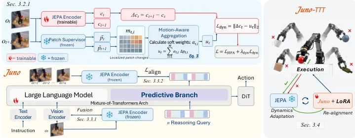
Figure 2: method overview (paper Fig. 3). Top left: Dynamic CLS pretraining aligns the trainable encoder's CLS transitions with motion-weighted patch changes from a frozen JEPA supervisor (Eqs. 3-4), under the total objective of Eq. 5. Bottom left: the Juno policy - a frozen JEPA encoder feeds patch fusion into the visual tokens, while a MoT predictive branch with K reasoning queries distills future CLS states (Eq. 6) jointly with the flow-matching action loss (Eq. 7). Right: Juno-TTT adapts the world model on all executions, successful and failed, then freezes the adapted teacher and re-aligns the policy on verified successes only. Flame and snowflake icons mark trainable and frozen modules.

Decoupled predictive reasoning: patch fusion plus MoT distillation

After pretraining the JEPA encoder is frozen and denoted $E_J$, and it keeps working in three places. First, patch-level fusion: current-frame patch features are projected to the VLA hidden width by a trainable two-layer MLP and fused into the native visual tokens through cross-attention with a gated residual connection of fixed gain $\gamma$, so spatial information enters the VLA while the original token sequence structure is preserved. Second, the predictive branch: instantiated as MoT decoder blocks in which the vision-language branch and the predictive reasoning branch keep separate non-embedding parameters while sharing one causal attention graph; the former preserves the representations used for action generation, the latter is dedicated to predicting future JEPA states. Third, the teacher role: K learnable reasoning queries are appended to the vision-language sequence; letting $H_{R,t}^L$ denote their final states, a trainable projector $g_r$ produces predicted future states $\widehat{Z}_t=g_r(H_{R,t}^L)$, while the frozen encoder supplies detached CLS targets from the K future observations, $Z_t^+=E_J^{\mathrm{cls}}(o_{t+\Delta:t+K\Delta})$. Because the number of queries matches the number of future targets, the alignment is one-to-one:

$$\mathcal{L}_{\mathrm{align}}=\frac{1}{BK}\sum_{b=1}^{B}\sum_{k=1}^{K}\left[1-\operatorname{cos}(\widehat{z}_{b,k},z^+_{b,k})+\lambda_{\mathrm{sl1}}\operatorname{SmoothL1}_\delta(\widehat{z}_{b,k},z^+_{b,k})\right], \tag{6}$$

with $\lambda_{\mathrm{sl1}}=\delta=0.1$ and $K=8$ queries matched to eight future frames at stride two. The crucial design point is the gradient pathway: the full hidden sequence, vision-language states plus reasoning states, conditions the flow-matching action decoder, so the reasoning branch receives both future-state alignment gradients and action-generation gradients. This joint pathway is what makes the aligned state decodable into actions rather than merely predictive of future observations. The joint objective is

$$\mathcal{L}_{\mathrm{VLA}}=\mathcal{L}_{\mathrm{FM}}+\alpha\,\mathcal{L}_{\mathrm{align}}, \tag{7}$$

where $\alpha$ follows a curriculum: linear warmup over W steps, a plateau of P steps, then half-cosine decay over D steps to 0.05 (5k/30k/70k for Bridge/Fractal and RoboCasa, with decay not quite reaching the floor inside the 100k-step budget). At inference the future-target path is removed and the predictive branch operates only on the current observation and the instruction.

The released code makes all three roles concrete. JEPAInputResidualFuser is a LayerNorm plus a scalar gate whose fusion weight is $\tanh(\text{gate})$, initialized at zero in the public config, so fusion starts switched off and learns its own strength. JEPAPatchCrossAttentionFuser applies LayerNorm to queries and keys, runs 8-head cross-attention, and scales the residual delta by a buffer (the paper text states $\gamma=0.2$; the public config sets input_xattn_scale: 0.5). The MoT decoupling is implemented in _make_mot_layer, which deep-copies each Qwen decoder layer's q/k/v/o projections, q_norm/k_norm, MLP, and both layer norms - guaranteeing matching shapes and dtypes while warm-starting the reasoning branch from pretrained weights - and in _make_mot_forward, which routes the last K tokens of the sequence through those copied parameters while attention itself remains a single joint attention over vision, language, and queries. detach_alignment_target=True keeps teacher targets gradient-free, and _curriculum_weight implements the $\alpha$ schedule of Eq. 7 verbatim. One discrepancy deserves a reviewer's attention: the paper text uses a plateau value of 1 for $\alpha$, whereas the public config sets align_loss_weight_max: 0.2, and a config comment notes that this "1005 working-tree" experiment uses a ViT-Base frozen-CLS target. The released recipe is therefore a variant of the paper system, not a verbatim reproduction.

flowchart TD
  TRAJ["embodiment-matched trajectories
BridgeData V2 + Fractal windows
4 frames stride 2, 14D action condition"] --> S1["Stage 1 control-aligned pretraining
LeWM ViT-Tiny ~15M, Eq.1
then frozen patch supervisor
Dynamic CLS Eq.2-4, L = L_JEPA + 0.2 L_dyn Eq.5"]
  S1 --> EJ["frozen JEPA teacher E_J
CLS c_t + patch grid P_t"]
  EJ --> FUSE["patch-level fusion
2-layer MLP + cross-attention
gated residual gain gamma"]
  EJ --> TEACH["detached future CLS targets
Z+ over K=8 future frames stride 2"]
  VLA["Qwen3-VL-4B visual+language tokens"] --> FUSE
  FUSE --> MOT["MoT decoupled reasoning branch
K learnable queries, shared causal attention
separate non-embedding params"]
  MOT --> ALIGN["one-to-one future distillation
L_align Eq.6 cosine + 0.1 SmoothL1"]
  MOT --> HID["full hidden sequence V+L+reasoning"]
  HID --> FM["flow-matching DiT action decoder
16-step chunks, 4 Euler steps"]
  FM --> LVLA["L_VLA = L_FM + alpha(s) L_align Eq.7
alpha: 5k warmup / 30k plateau / 70k decay to 0.05"]
  ALIGN --> LVLA
  TEACH --> ALIGN
  LVLA --> POL["frozen Juno policy"]
  POL --> ROLL["deployment rollouts
D_ok verified success + D_fail failures"]
  ROLL --> TTT1["Juno-TTT stage 1 Eq.8
full-param world-model update on D_ok + D_fail
10 epochs AdamW 1e-6"]
  TTT1 --> EJ2["frozen adapted teacher E_J^ttt"]
  EJ2 --> TTT2["Juno-TTT stage 2 Eq.9
policy re-aligned on D_ok only
LoRA rank 32 + trainable action head, 400 steps"]
  TTT2 --> ADAPT["adapted policy Juno-TTT"]

Figure 2 supplement: data flow of the three-stage pipeline. The same action-conditioned JEPA is first control-aligned on embodiment-matched trajectories, then frozen to serve simultaneously as fusion source and future-state teacher; at deployment it is unfrozen once more, adapted on every transition including failures, and refrozen as the teacher while the policy is re-aligned on verified successes only.

Dynamics-first test-time adaptation: failures teach only the world

Control-aligned pretraining and decoupled reasoning already yield strong frozen policies that tolerate moderate shifts in background, layout, and object instance. Under harsher shifts - strong observation noise or abrupt illumination change - the frozen teacher itself becomes unreliable and the coupled policy collapses. Juno-TTT starts from a single observation: a failed action cannot teach the robot what to do, but faithfully witnesses how the world responds. A failed rollout still records truthfully how the executed actions changed the environment, and those transitions can be exploited without expert corrections or task rewards. The deployment buffer is cleaned into two disjoint subsets, transitions from verified successful executions $\mathcal{D}_{\mathrm{ok}}$ and transitions from failed executions $\mathcal{D}_{\mathrm{fail}}$ (a lightweight procedure removes invalid segments), with the full buffer written $\mathcal{D}_{\mathrm{ttt}}=\mathcal{D}_{\mathrm{ok}}\cup\mathcal{D}_{\mathrm{fail}}$.

Stage 1, dynamics adaptation, performs a full-parameter update of $f_\theta$ and $g_\phi$ from their pretrained weights on the entire buffer, using the same action-conditioned objective as pretraining:

$$\theta^\star,\phi^\star=\arg\min_{\theta,\phi}\;\mathbb{E}_{(o_t,a_t,o_{t+1})\sim\mathcal{D}_{\mathrm{ttt}}}\Big[\mathcal{L}_{\mathrm{pred}}\big(g_\phi(c_t,a_t),\,c_{t+1}\big)+\lambda_{\mathrm{reg}}\mathcal{R}(c)\Big], \tag{8}$$

This objective supervises only the consequences of executed actions, so failed trajectories provide exactly the same learning signal as successful ones at this stage. Stage 2, policy re-alignment, freezes the adapted encoder $E_J^{\mathrm{ttt}}\triangleq f_{\theta^\star}$, which replaces the original teacher and supplies future targets $\widetilde{Z}_t^+=E_J^{\mathrm{ttt,cls}}(o_{t+\Delta:t+K\Delta})$; the policy is then re-aligned on verified executions only, with the same composite objective as training:

$$\mathcal{L}_{\mathrm{ttt}}(\psi)=\mathbb{E}_{\mathcal{D}_{\mathrm{ok}}}\Big[\mathcal{L}_{\mathrm{FM}}(\psi)+\lambda_{\mathrm{ttt}}\,\mathcal{L}_{\mathrm{align}}(\psi;\widetilde{Z}^+)\Big]. \tag{9}$$

For stability under scarce test-time data, the policy is updated through LoRA adapters (rank 32, alpha 64, dropout 0.05, applied to attention and MLP projections of the backbone and predictive branch) while pretrained backbone weights stay frozen; the action head is fully trainable without LoRA, and all test-time updates use reduced learning rates (stage 1: 10 epochs of AdamW at 1e-6; stage 2: 400 steps with 5e-7 for backbone LoRA adapters and 5e-6 for the other adapters and the action head, 10-step warmup and cosine decay to 5e-8). The asymmetry between stages is the sharpest line in the paper: dynamics adaptation consumes every transition, while policy re-alignment trusts only verified executions - failed actions never become imitation targets - and freezing $E_J^{\mathrm{ttt}}$ keeps the alignment target fixed throughout policy adaptation.

Experiments

Benchmarks and implementation details

Three fronts cover simulation and hardware. SimplerEnv (WidowX): policies train on BridgeData V2 and Fractal in LeRobot format (53,192 and 87,212 episodes; the sampler picks a source with probability 1/2 then draws an episode and timestep uniformly within it), with a single 224x224 RGB view, 16-step action chunks, and eight future frames at stride 2 for latent alignment; reported numbers are means over four evaluation runs. RoboCasa-GR1 Tabletop: one multitask policy over 24 tasks with equal task-sampling weights, ego-view RGB without proprioception, 29-channel actions (two arms, two hands, waist), 50 episodes per task at evaluation. Real robot: the right PiPER arm of an AgileX Cobot Magic ALOHA-style leader-follower platform, fine-tuned from the SimplerEnv policy on 60 demonstrations of "put the red cube into the blue bowl" (20 at each of three fixed cube positions); evaluation runs 20 trials per condition and every condition, including in-domain, uses cube positions held out from the demonstration placements; deployment runs at 15 Hz executing the full 16-step chunk (about 1.07 s) before the next observation and replan, with increments converted by damped least-squares inverse kinematics and actions skipped when the IK residual exceeds 0.01 m or 0.10 rad. Optimization: all three recipes share Qwen3-VL-4B-Instruct with a GR00T flow-matching decoder, AdamW (0.9, 0.95), cosine decay to 5e-7, BF16, and DeepSpeed ZeRO-2; Bridge/Fractal and RoboCasa run 100k steps with global batch 128 and 64, backbone at 1e-5 and predictive branch and action decoder at 1e-4; PiPER fine-tuning runs 50k steps with LoRA at 1e-4 on backbone and predictive branch and 1e-5 on the action decoder.

SimplerEnv: +7.6 over the strongest baseline, +11.8 after adaptation

Method	Average	Spoon on towel	Carrot on plate	Stack green block	Eggplant in basket
OpenVLA-OFT	41.8	34.2	30.0	30.0	72.5
CogACT	51.3	71.7	50.8	15.0	67.5
VideoVLA	53.1	75.0	20.8	45.8	70.8
pi-0	53.1	29.2	62.5	29.2	91.6
VLA-JEPA	57.3	75.0	70.8	12.5	70.8
pi-0.5	57.1	49.3	64.7	44.7	69.7
Isaac-GR00T-N1.6-Bridge	57.1	64.5	65.5	5.5	93.0
Qwen3GR00T	60.9	72.9	60.4	14.6	95.8
Juno	68.5	86.5	59.4	31.3	96.9
Juno-TTT	72.7	94.8	62.5	37.5	95.8

Table 1: SimplerEnv (WidowX) success rates in percent, excerpted from paper Table 1 (means over four runs). Juno improves on the strongest baseline Qwen3GR00T by 7.6 points on average, with gains concentrated where the baseline is weakest - block stacking from 14.6 to 31.3 and spoon placement from 72.9 to 86.5. Carrot placement is one of the few cells where Juno trails: 59.4 against 60.4 for Qwen3GR00T and 70.8 for VLA-JEPA. TTT raises the average to 72.7 in the nominal condition, showing that even without distribution shift the policy's own rollouts provide useful dynamics supervision.

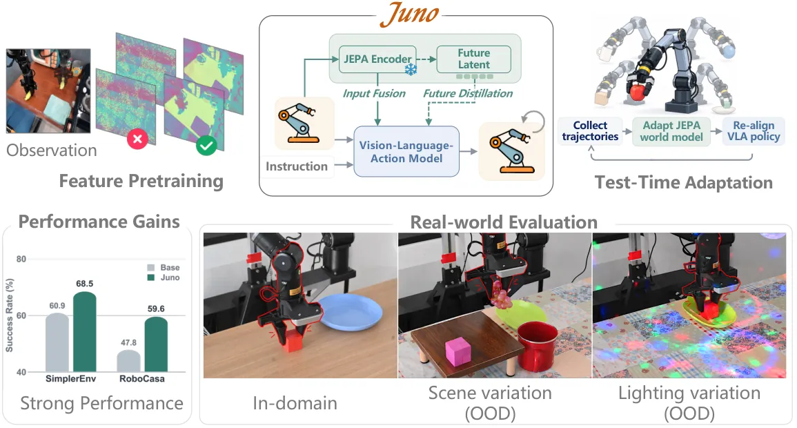
Figure 3: full-paper overview (paper Fig. 1). Top row: the three roles - feature pretraining over observations and patch maps, the Juno core in which a JEPA encoder and future latent feed the VLA through input fusion and future distillation, and test-time adaptation as a collect-adapt-realign loop. Bottom left: success bars, 60.9 to 68.5 on SimplerEnv and 47.8 to 59.6 on RoboCasa. Bottom right: real-robot snapshots for in-domain, scene-variation, and lighting-variation conditions.

RoboCasa-GR1: winning 21 of 24 tasks

Method	PnP+Close	Cuttingboard	Placemat	Plate	Tray	Average
GR00T-N1.6	24.2	56.9	51.9	57.6	55.1	47.6
Qwen3PI	42.3	46.0	43.5	44.0	44.0	43.9
Qwen3OFT	43.7	50.4	41.5	61.0	49.2	48.8
Qwen3FAST	35.0	50.4	33.5	45.0	32.0	39.0
Qwen3GR00T	50.3	52.8	38.0	58.5	39.2	47.8
Juno	57.3	64.8	55.5	68.0	53.6	59.6

Table 2: RoboCasa-GR1 Tabletop unweighted mean success per task group in percent (paper Table 2; the average column is over all 24 tasks). Juno reaches 59.6 against 47.8 for Qwen3GR00T and 48.8 for Qwen3OFT, taking first place in four of five groups and winning 21 of the 24 individual tasks. The Tray group, 53.6 against 55.1 for GR00T-N1.6, is the only group-level deficit.

Real robot: frozen-policy robustness under cumulative shifts

Method	In-domain	Background	+ Height	+ Height + Object
Qwen3GR00T	40.0 (8/20)	0.0 (0/20)	0.0 (0/20)	0.0 (0/20)
Juno	100.0 (20/20)	75.0 (15/20)	70.0 (14/20)	70.0 (14/20)

Table 3: frozen-policy real-world evaluation (paper Table 3), 20 trials per condition, with cumulative shifts: tablecloth, cube color, and bowl shape/color change first; the work plane is then raised by 10 cm; finally the cube is replaced by a grape and the instruction updated. Juno scores 20/20 in-domain against 8/20 for the baseline, a 60-point gap, and retains 75/70/70 across the three shifted conditions while the baseline collapses to zero in all of them. Both policies are frozen here, so the gains are attributable to the learned representations alone.

Method	Gaussian observation noise	Dynamic lighting
Juno (frozen)	40.0 (8/20)	55.0 (11/20)
+ Juno-TTT	65.0 (13/20)	70.0 (14/20)

Table 4: real-robot test-time training (paper Table 4), with 40 rollouts collected and adapted separately per condition. Success rises from 40 to 65 under Gaussian observation noise and from 55 to 70 under dynamic lighting: the harsher the shift, the larger the marginal value of deployment data, consistent with the claim that failed transitions are valid dynamics supervision.

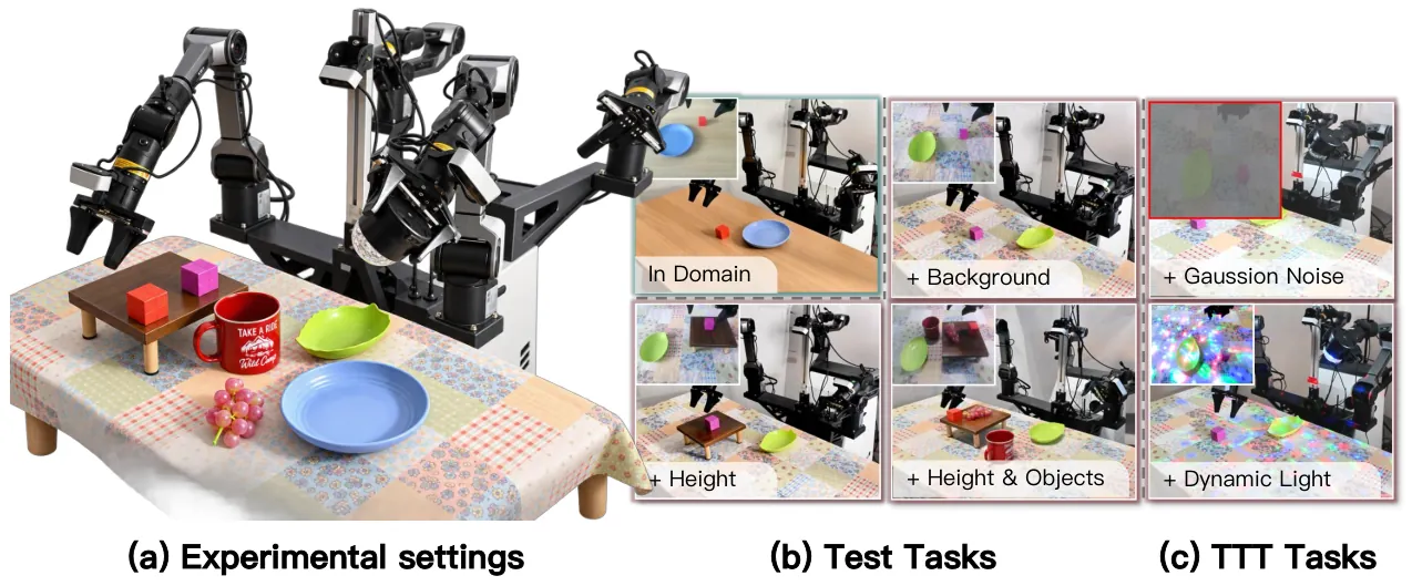
Figure 4: real-robot setup and conditions (paper Fig. 4). (a) The AgileX Cobot Magic platform with only the right PiPER arm used. (b) Cumulative shift conditions for the frozen policy: in-domain, +background, +height, +height and object. (c) The two test-time training conditions: Gaussian observation noise and dynamic colored lighting.

Ablation: fusion and MoT are a coupled pair

Patch fusion	MoT branch	L_align	L_dyn	Average success
removed	yes	yes	yes	53.9 (-14.6)
yes	removed	yes	yes	65.4 (-3.1)
yes	yes	removed	yes	60.8 (-7.7)
removed	removed	yes	yes	60.4 (-8.1)
yes	yes	yes	removed	65.6 (-2.9)
yes	yes	yes	yes	68.5

Table 5: leave-one-out component ablation on SimplerEnv (paper Table 5). Removing patch fusion alone causes the largest drop, 53.9, below the 60.9 base VLA; removing fusion together with the MoT branch recovers to 60.4, because without the grounded patch pathway the predictive branch imposes future-state objectives on ungrounded representations and turns harmful. Removing the MoT branch alone costs only 3.1 points, so its value is realized through fusion. Without L_align the model gains nothing over the base VLA (60.8 versus 60.9): the predictive branch helps only when its predictions are directly supervised. The Dynamic CLS loss contributes a smaller but consistent gain (-2.9).

Representation analysis: why the teacher qualifies

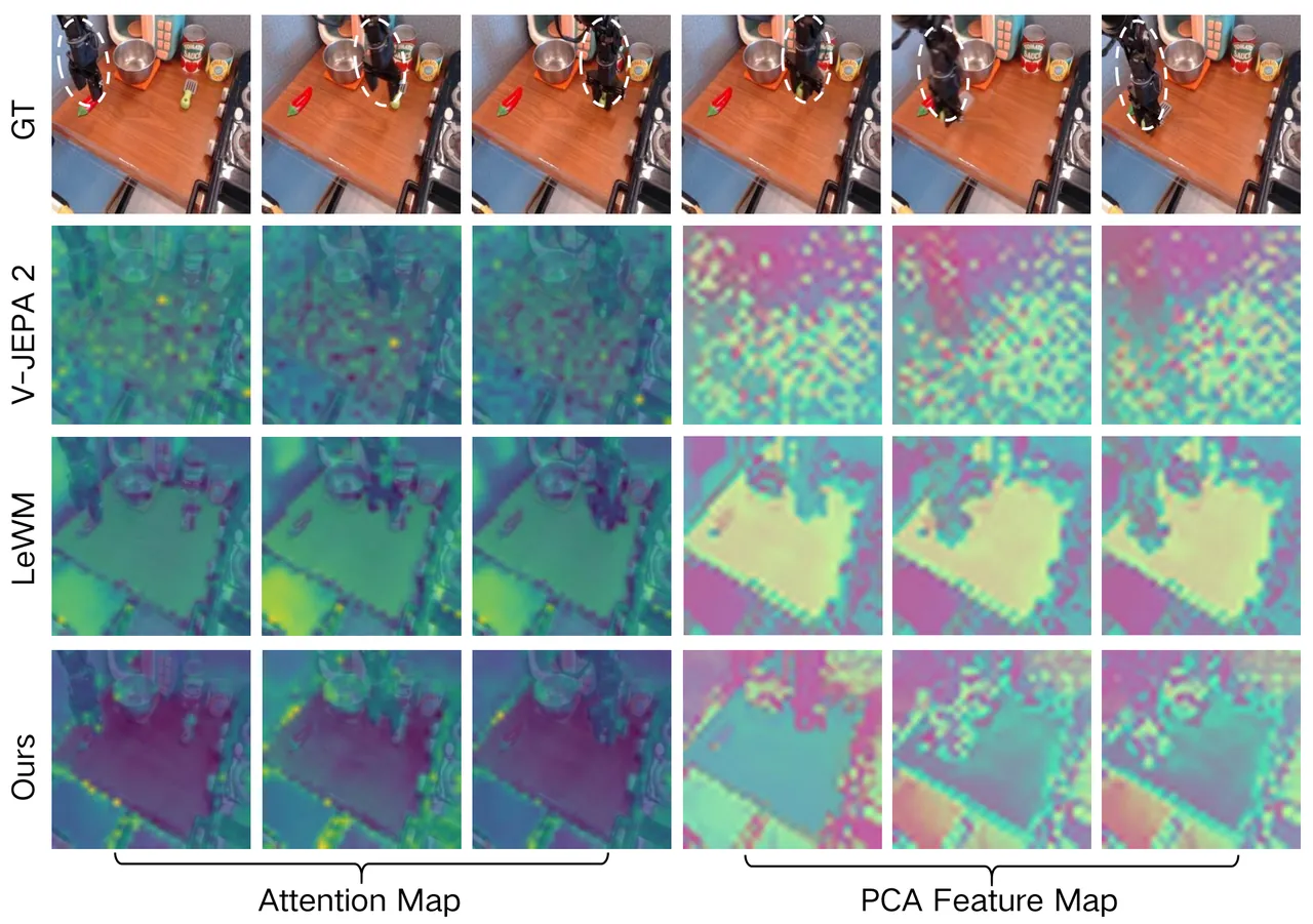
Figure 5: spatial feature structure (paper Appendix A, Fig. 5). Below the ground-truth row come V-JEPA 2, LeWM, and the control-aligned encoder trained with the Dynamic CLS loss. V-JEPA 2 spreads attention across the scene with fine-scale PCA variation; LeWM concentrates on the manipulation region and separates robot, bowl, and object from the tabletop; the control-aligned encoder shows still more concentrated attention along robot and object boundaries while retaining the foreground-background separation. PCA is fitted separately per encoder, so colors are comparable only within one encoder.

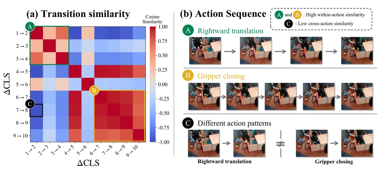
Figure 6: CLS transition similarity (paper Appendix A, Fig. 6). (a) Pairwise cosine similarity of the nine transition vectors delta c_t = c_{t+1} - c_t: the green block A (rightward-translation transitions 1-2 through 3-4) and the yellow block B (gripper-closing transitions 6-7 through 9-10) are warm within themselves, while the black-outlined cell C contrasting a translation with a closing transition is cold. (b) The corresponding observation sequences. Global-token changes therefore distinguish action patterns while staying consistent within each pattern, which is exactly the motivation of the Dynamic CLS loss.

Limitations and Open Questions

First, the interpretive boundary of the representation analysis (author-stated). Appendix A states explicitly that the comparisons "assess teacher suitability in the studied control setting and do not isolate pretraining data, architecture, and objective as independent factors"; that the attention and PCA maps "indicate where information is represented" but "do not identify the pixels used by the downstream policy"; and that the transition-similarity matrix concerns transition direction in representation space, does not measure transition magnitude, and does not by itself isolate the effect of the loss. The causal evidence for "control alignment" therefore remains indirect.

Second, scale and embodiment coverage (author-stated). The conclusion defers to future work the scaling of training and evaluation across larger datasets, broader tasks, and multiple embodiments. The real-robot evidence rests on a single platform and a single task family with 60 demonstrations, and each simulation benchmark uses one action-space configuration. Claims about frozen-policy shift robustness are therefore established on a narrow slice of single-arm tabletop manipulation.

Third, coupling-induced tuning fragility. The ablation shows patch fusion and the MoT branch behave as a coupled pair: removing fusion alone drops performance to 53.9, below the component-free 60.9, while removing both recovers to 60.4; removing L_align erases the predictive branch's benefit entirely. The predictive branch is a net negative without a grounded pathway or direct supervision, so all three components must be present simultaneously - an expensive tuning constraint for anyone reusing this architecture.

Fourth, TTT is an offline protocol that depends on success verification. Juno-TTT first collects a fixed set of rollouts, runs the two adaptation stages offline, and evaluates the adapted policy frozen; it is not online continual adaptation. The SimplerEnv TTT result is measured in the nominal condition only, to isolate the value of deployment data absent shift, so shift-conditioned evidence comes solely from the two real-robot settings. Stage 2 additionally requires the external judgment of "verified successful executions" (a lightweight cleaning step removes invalid segments); if the success/failure criterion is unreliable, the partition into D_ok and D_fail writes that error into both teacher and policy.

Fifth, the public reproducibility boundary. The repository releases only the Bridge/Fractal policy-learning stage; JEPA pretraining code, TTT code, and checkpoints remain unchecked in the README TODO, and docs/reproducibility.md states that README scores are reported paper results that should not be attributed to this code before running the prescribed data split and evaluation protocol. Auditable differences between the public config and the paper text (alignment weight cap 0.2 versus 1, cross-attention scale 0.5 versus 0.2, ViT-Base frozen-CLS target versus the ViT-Tiny teacher) mean verbatim reproduction of the paper numbers requires additional unreleased assets.

Conclusion and Outlook

Juno's contribution is not yet another world-model interface but the discipline of using one action-conditioned JEPA as three different tools. During pretraining the Dynamic CLS loss shapes it so that a compact CLS state carries patch-level motion; during policy learning it freezes into a teacher whose patch fusion and decoupled MoT branch distill future states into action generation, with alignment gradients and action gradients meeting in the same hidden sequence; at deployment it unfreezes once more, absorbing every transition including failures as dynamics supervision before refreezing as the teacher that only verified successes may touch. The evidence chain - 68.5 on SimplerEnv (72.7 after TTT), 59.6 on RoboCasa-GR1, frozen real-robot scores of 100/75/70/70 against a baseline's 40/0/0/0, plus ablations and TTT gains consistent with "failures teach only the world" - supports the paper's central claim that predictive latents must be tamed by the control problem to be useful at all. The released policy-stage code and its auditable config keep the verification bar comparatively low for this class of work. The open questions are equally clear: whether control alignment survives scaling across embodiments, whether test-time adaptation can be made online and freed from external success verification, and whether a latent-space teacher of this kind can grow the high-fidelity futures needed for planning and inspection.