Action-Aligned Latent Planning for Versatile Humanoid Loco-Manipulation

Paper Metadata

Title: Action-Aligned Latent Planning for Versatile Humanoid Loco-Manipulation (FIBER)

Authors: Yutang Lin, Guanya Shi^†, C. Karen Liu^† (^†Amazon FAR Team Co-Leads). Affiliations: Amazon Frontier AI & Robotics, Carnegie Mellon University, Stanford University.

Links: arXiv:2610.24675 (v2, 2026-10-20, cs.RO, CC BY 4.0) · arXiv HTML full text · project page · overview video

Code status: ⏳ Pending release. github.com/Yutang-Lin/FIBER (Apache-2.0, created 2026-10-20, roughly 14 MB) currently ships only the teaser image, the pipeline figure, a demo GIF, badges, links and BibTeX. The README states plainly: Code coming soon. This repository currently contains the paper's teaser, visual overview, links, and citation. There is no training code, no inference code and no checkpoint. The project page does host an in-browser MuJoCo playground where real-robot rollouts can be inspected interactively.

Background and Motivation

Humanoid loco-manipulation couples two problems that are usually solved separately. The first is a decision problem: look at a scene and determine which interaction to initiate. The second is a control problem: realize that interaction through balance, contact and coordinated whole-body actuation. Task-specific interaction skills have become genuinely good — object manipulation, articulated-object interaction and object transport all have strong published policies — but nearly all of them are built on task-specific objectives, task-specific observation spaces and task-specific training procedures. Assembling such specialists into one versatile policy is therefore not a matter of adding output heads. The hard question is what representation should sit between high-level planning and whole-body control.

The conventional answer is hierarchical: a high-level policy predicts structured targets such as body motion, end-effector poses or contact sequences, and a low-level controller realizes them on hardware. The paper states the failure mode of this design unusually bluntly. The same target can require entirely different actions under different contacts, object states or disturbances, so a kinematic or contact abstraction simply does not encode the state-dependent control response that makes an interaction succeed. The authors back this with a sharp piece of evidence: FALCON, which explicitly learns force-adaptive end-effector tracking under randomized external forces, still reaches only 0.4% (with approach) and 2.7% (without approach) on door opening. A tracker that already knows how to modulate force cannot recover task-specific interaction responses.

The opposite extreme — having the planner predict low-level actions directly — removes the abstraction but inherits an impossible data requirement. Offline learning must then cover a broad distribution of closed-loop corrective responses, which for contact-rich interaction is effectively out of reach. The paper's Action Planner baseline is exactly this design, and it scores 0.0% on all three tasks. The reason is arithmetic as much as statistical: at a 5 Hz planning rate, ten body-control steps elapse between planner updates, and a raw action chunk carries no state feedback whatsoever across that gap.

This gives the paper its central question, worth stating verbatim: how can we abstract low-level control complexity without abstracting away the physical responses that make interaction succeed? The proposed resolution is to stop looking for a representation of the desired motion and instead use a representation that already indexes a policy. A BFM latent command $z$, evaluated against the current robot state $s_t$ at 50 Hz, produces low-level actions; so $z$ denotes a state-dependent control policy rather than a trajectory. High-level planning can then operate over compact behavioral commands at a low rate while the frozen BFM continues to supply high-frequency closed-loop physical feedback.

An interface alone is not enough — the planner still needs interaction capabilities to invoke. Two standard routes for acquiring them are both rejected here for concrete reasons. Collecting demonstrations through a common data-acquisition pipeline is expensive precisely where it matters most, since broad coverage of contact-rich and corrective behavior is what such pipelines struggle to produce. Distilling task-specific experts into a generalist works better on paper, and on-policy multi-expert distillation genuinely improves closed-loop coverage by querying experts at states the generalist actually visits — but it requires every expert policy and every expert environment to remain available throughout integration. The authors instead adopt a deliberately looser, decoupled setting: each interaction policy is acquired independently, and only afterwards incorporated into the shared behavioral interface. This matches how robot skill libraries are actually built, where a box-carrying group and a door-opening group may work in different codebases with different observation spaces and never need to be co-resident.

Decoupling produces the observation the whole method rests on. Experts that share nothing else — different supervision, different observations, different objectives, different action normalization conventions — nevertheless share one quantity that directly describes their physical realization: the actions applied to the robot. A frozen BFM latent command is grounded in the same quantity, because it too produces robot actions conditioned on the current state. That common action space is the bridge between an independently acquired interaction policy and the BFM latent representation, and it is where the phrase action-aligned in the title comes from.

Preliminaries: An Executable Latent Space and Forward-Backward Representations

FIBER builds on the BFM-Zero line of work, which uses forward-backward (FB) representations to learn a promptable humanoid behavioral space. For a latent-conditioned policy, the forward representation admits a successor-feature interpretation:

$$F_{\gamma}(s_{t},a_{t},z)\approx\mathbb{E}\left[\sum_{h=0}^{\infty}\gamma^{h}B(s_{t+h+1})\;\middle|\;s_{t},a_{t},\pi_{\mathrm{BFM}}(\cdot,z)\right]$$

with FB value $Q_{\gamma}^{\mathrm{FB}}(s,a,z)=F_{\gamma}(s,a,z)^{\top}z$. Read informally, $z$ selects a behavioral direction and $B(s)$ gives the coordinates of a state in that behavioral basis, so their inner product is the long-horizon value of the indexed policy at that state. One consequence is used heavily later in the paper: because $B(s)$ is both a value component and a state descriptor, it can serve as a native semantic label for the current state. That is the ingredient behind the semantic regularizer in LPP.

Executable body commands are constrained to a fixed-radius sphere with projection operator

$$\mathcal{Z}=\left\{z\in\mathbb{R}^{d_{z}}:\|z\|_{2}=\sqrt{d_{z}}\right\},\qquad \Pi_{\mathcal{Z}}(v)=\sqrt{d_{z}}\,\frac{v}{\|v\|_{2}}$$

The paper uses $d_{z}=256$ and notes that the fixed-radius parameterization keeps the average squared coordinate magnitude independent of the latent dimension; a fixed nonzero reference vector handles the degenerate zero-norm case. This constraint is global: projector outputs, $B$ outputs and planner samples all pass through $\Pi_{\mathcal{Z}}$. Two corollaries recur throughout the method. Interpolation in this space must be spherical rather than linear, and squared distance reduces to a cosine gap up to a constant factor — an identity the paper writes out explicitly.

On the control side, the BFM body action is 29-dimensional: the 29 actuated joints of the Unitree G1 at 50 Hz with control interval $\Delta t=0.02$ s. Tasks using Dex3 hands additionally predict 14 hand-joint targets (seven per hand), produced by a separate branch that is not part of the BFM body action — a detail that turns out to matter when interpreting the grasping results. The actor consumes the current proprioceptive state

$$s_{t}^{\mathrm{prop}}=\left[q_{t}-q^{\mathrm{default}};\ \dot{q}_{t};\ g_{t}^{\mathrm{body}};\ 0.25\,\omega_{t}^{\mathrm{body}}\right]\in\mathbb{R}^{64}$$

where $g^{\mathrm{body}}$ is the gravity direction and $\omega^{\mathrm{body}}$ the body angular velocity, together with the previous scaled body action and nine causal proprioceptive/action history frames of 93 entries each (29 action, 3 angular velocity, 29 joint position, 29 joint velocity, 3 gravity). The actor therefore receives $64+29+9\times 93=930$ proprioceptive and action coordinates before the latent command is appended. The backward representation additionally receives 463 dimensions of heading-frame whole-body kinematics during BFM training and simulation-based projection, but the deployed BFM actor consumes none of these privileged quantities. That boundary is what makes the real-robot claim meaningful: the controller running on hardware is a pure proprioceptive policy.

Method

FIBER proceeds in three stages. Interaction skills are first acquired independently with task-appropriate supervision. LPP then maps each expert into the frozen BFM latent space by matching the actions induced by latent commands to the expert's local control responses. The projected policies are rolled out directly through the shared behavioral interface, after which — the paper says this twice, and it is the load-bearing claim of the decoupled design — the original experts are no longer required. Finally the closed-loop latent rollouts are aggregated to train a single perceptive flow planner entirely offline, conditioned on onboard observations and a high-level steering command. The diagram below follows the real structure of Fig. 1 and Appendices A-D, and highlights the two frequency domains plus the feedback edge from BFM back into the loop, which is what separates FIBER from direct action planning.

flowchart TB
    subgraph ACQ["Stage 1 Acquisition - three independent routes"]
        A1["Motion imitation experts
box pickup and object grasping
HDMI style, privileged encoder 256-d"]
        A2["Staged reward shaping expert
door opening: approach, contact,
handle manipulation, open"]
        A3["SF guided behavior reuse
carry composed with crouch, kneel,
walk, run by swapping z_N"]
    end
    subgraph PROJ["Stage 2 LPP - action aligned latent policy projection"]
        B1["Projector P_psi_i : pre-norm residual MLP
width 1024, 4 blocks motion / 2 blocks door"]
        B2["Sphere SLERP between updates
10 Hz projector, H_P = 5 body steps"]
        B3["L_act on physical joint targets
plus 0.1 x L_sem anchoring z_k to B of s"]
        B4["Single skill on-policy data aggregation
DAgger style, executed latent noise std 0.1"]
    end
    subgraph PLAN["Stage 3 unified offline latent flow planning"]
        C1["20K closed loop episodes per skill
depth 144x256 plus proprio 58
plus condition plus executed z"]
        C2["Conditional DiT flow planner
width 1024, 16 blocks, 8 heads
H = 10 latents covering 1 s"]
        C3["Steering encoder, 2 blocks
frozen T5-base 768-d language
10-d waypoint, 8 output tokens"]
    end
    BFM["Frozen AH-BFM
d_z = 256 sphere, multi-gamma FB
50 Hz, 29 joint targets, about 1 ms"]
    ROBOT["Unitree G1 driven by a single
RTX PRO 5000 Blackwell laptop"]
    A1 --> B1
    A2 --> B1
    A3 --> B1
    B1 --> B2 --> B3 --> B4
    BFM --> B3
    B4 --> C1 --> C2
    C3 --> C2
    C2 -->|future 1 s of latents, replan 5 Hz, about 20 ms| BFM
    BFM -->|high rate state dependent feedback, never modeled by the planner| ROBOT
    B4 -.->|experts discarded once projection finishes| GONE["no expert environment needed for planner training"]

Figure 1: The three-stage FIBER dataflow, drawn from the paper's Fig. 1 and Appendices A-D. Two properties deserve attention: experts are discarded after projection, and deployment couples a 5 Hz planner to a 50 Hz frozen controller.

1. Adaptive-Horizon BFM: One Latent Space, Two Temporal Requirements

Projection and planning impose contradictory demands on the same latent representation. LPP must reproduce an expert's local control response inside a 0.1 s window, which favors a short successor horizon. A 5 Hz planner wants a single latent command to preserve one coherent behavior over a much longer interval, which favors a long horizon. Conventional FB learning forces a choice, and the paper identifies this as a genuine trade-off rather than a tuning nuisance. AH-BFM resolves it by treating the discount as a conditioning variable:

$$\Gamma=\{\gamma_{s},\gamma_{l}\},\qquad \gamma_{s}<\gamma_{l}$$

The forward representation $F$ is conditioned on $\gamma$ (embedded by a small MLP before entering the forward network, and deliberately not fed to the actor), while the backward map $B$ and the executable actor are shared across horizons. Values at different discounts have different natural scales, so they are normalized first:

$$\widetilde{Q}_{\gamma}^{\mathrm{FB}}=(1-\gamma)\,Q_{\gamma}^{\mathrm{FB}},\qquad V_{\gamma}(s,z)=(1-\gamma)\,Q_{\gamma}^{\mathrm{FB}}\bigl(s,\pi_{\mathrm{BFM}}(s,z),z\bigr)$$

The $(1-\gamma)$ factor removes the leading discounted-sum scale and makes short- and long-horizon terms directly comparable. The shared actor then maximizes a log-sum-exp aggregation rather than a weighted sum:

$$J_{\mathrm{FB}}(s,z)=\tau\log\sum_{\gamma\in\Gamma}p(\gamma)\exp\!\left(\frac{V_{\gamma}(s,z)}{\tau}\right)$$

whose gradient decomposes into a convex combination of horizon-specific policy gradients with weights that depend on the current state and latent command rather than being fixed globally:

$$w_{\gamma}(s,z)=\frac{p(\gamma)\exp\!\bigl(V_{\gamma}(s,z)/\tau\bigr)}{\sum_{\gamma^{\prime}\in\Gamma}p(\gamma^{\prime})\exp\!\bigl(V_{\gamma^{\prime}}(s,z)/\tau\bigr)}$$

In practice $\Gamma=\{0.8,\,0.98\}$ with prior $p(0.8)/p(0.98)=0.625/0.375$ and aggregation temperature $\tau=1$. Appendix A-C devotes real space to justifying the aggregator: it is non-expansive in $\|\cdot\|_{\Gamma,\infty}$, and — the property the authors stress — it does not amplify perturbations introduced through the FB backup, since the composed operator contracts at rate $\gamma_{\max}=\max\Gamma<1$. A separate subsection contrasts it with the fixed weighted-sum objective $J_{\mathrm{WS}}(s,z)=\sum_{\gamma}p(\gamma)V_{\gamma}(s,z)$, which cannot switch the dominant horizon as a function of state.

2. Three Acquisition Routes: Only the Actions Have to Match

The immediate payoff of decoupling is that experts may be trained however the task suggests. The paper uses three complementary routes. Motion-based acquisition covers interactions with suitable humanoid-object motion references, namely grasping and pickup: an HDMI-style expert with a privileged observation encoder producing a 256-dimensional embedding and a reference-action residual actor, actor hidden widths [512, 256, 256], critic widths [512, 256, 128], Mish activations, and PPO at learning rate $3\times10^{-4}$, 3 epochs, 8 minibatches, clip 0.2, discount 0.99, GAE 0.95, entropy coefficient 0.001. Tracked quantities include both body motion and manipulated-object pose, with contact rewards forcing the demonstrated interaction to be realized physically. Reward-shaping-based acquisition covers interactions that decompose into successive stages: door opening is trained by progressively rewarding approach, contact establishment, handle manipulation and opening, needing no motion reference at all and letting each stage use its own observations and rewards.

The third route is the most interesting because it attacks combinatorial explosion. Carrying a box while crouching, kneeling, walking or running would each need a separate motion reference or a separate expert under conventional pipelines. Instead the BFM is frozen and only a latent adapter is learned:

$$\hat{z}_{t}=\Pi_{\mathcal{Z}}\!\left(z^{N}+A_{\psi_{I}}^{\mathrm{res}}(o_{t},z^{N})\right),\qquad a_{t}=\pi_{\mathrm{BFM}}(s_{t},\hat{z}_{t})$$

The residual parameterization lets the adapter modify the native command $z^{N}$ only as much as the interaction requires. Training uses the interaction reward plus a successor-feature preservation term:

$$r_{t}=r_{t}^{I}+\lambda_{\mathrm{SF}}\,B(s_{t})^{\top}z^{N}$$

Because $z^{N}$ is fixed, $\mathbb{E}\bigl[\sum_{t}\gamma^{t}B(s_{t})^{\top}z^{N}\bigr]=\mathbb{E}\bigl[\sum_{t}\gamma^{t}B(s_{t})\bigr]^{\top}z^{N}$, so the second term evaluates the discounted state occupancy along the behavioral direction selected by $z^{N}$. Since both $B(s_t)$ and $z^{N}$ lie on the radius-$\sqrt{d_z}$ sphere, $B(s_{t})^{\top}z^{N}/d_{z}=\cos\angle\bigl(B(s_{t}),z^{N}\bigr)$, meaning the normalized and unnormalized forms differ only by a constant absorbed into $\lambda_{\mathrm{SF}}$. The paper flags one easy mistake explicitly: the preservation target is the requested native behavior $z^{N}$, not the adapted latent $\hat{z}_t$; reversing this makes the adapter self-referential. For the carrying compositions, $r^I$ contains upper-body pose, object position, object orientation and contact terms with weights 1, 2, 1 and 1, using kernels $r_{\mathrm{pose}}=\exp(-e_q/0.25^2)$, $r_{\mathrm{pos}}=\exp(-\|e_p\|_2^2/0.10^2)$ and $r_{\mathrm{ori}}=\exp(-\theta_{\mathrm{obj}}^2/0.35^2)$; the SF term carries weight 0.1, a latent-smoothness cost $c_{\mathrm{smooth},t}=\|\hat{z}_{t}-\hat{z}_{t-1}\|_{2}^{2}/(2d_{z})$ — exactly one minus cosine similarity on $\mathcal{Z}$ — carries weight $-0.5$, and object-drop termination contributes $-100$. Adapter actor and critic use two residual feed-forward blocks of width 512 with feed-forward width 2048 and GELU activations; the SF adapter runs at learning rate $10^{-5}$ for 5 epochs.

3. Latent Policy Projection: The Technical Core

Once an expert exists, it must be converted into something an offline planner can be trained on. Kinematic trajectories are compact but do not uniquely determine the control responses an interaction requires. Expert actions carry exactly that missing physical information, yet modeling high-frequency actions directly demands covering a broad state-dependent control distribution. LPP takes the middle path: use the frozen BFM to compress expert behavior into a lower-rate latent representation that retains both its executable response and its native behavioral semantics.

Alignment has to happen in a shared physical space, because different experts use different normalized action conventions. Both BFM and expert outputs are therefore converted to physical body joint targets first. Under the BFM control profile,

$$q_{t}^{\mathrm{des}}=q^{\mathrm{default}}+0.25\,r_{q}\odot\operatorname{clip}\!\left(6a_{t},-6,6\right)$$

where $r_q$ holds per-joint action scales. Joint order, default pose and scale vectors are kept consistent across expert conversion, projection, projected-rollout collection and execution, and the resulting targets are realized by the robot PD controller with the gains and actuator limits of the selected profile. Comparing physical joint targets — rather than normalized actions — is what prevents one expert's convention from silently changing the meaning of the alignment loss.

For expert $\pi_i^{E}$, a local projector $P_{\psi_i}$ maps the expert observation at update time $t_k$ to a latent command $z_{k}=P_{\psi_{i}}(o_{t_{k}}^{E_{i}})\in\mathcal{Z}$. Projection updates occur every five body-control steps, a 0.1 s interval corresponding to a 10 Hz projector; between updates the command is interpolated on the sphere:

$$z_{t_{k}+h}=\operatorname{SLERP}\!\left(z_{k-1},z_{k},\alpha_{h}\right),\quad h=0,\ldots,H_{P}-1,\qquad H_{P}=5$$

$$\operatorname{SLERP}(a,b,\alpha)=\frac{\sin\!\bigl((1-\alpha)\vartheta\bigr)}{\sin\vartheta}\,a+\frac{\sin\!\bigl(\alpha\vartheta\bigr)}{\sin\vartheta}\,b$$

with $\vartheta$ the angular separation between endpoints and its cosine clamped for numerical stability. The projector itself is a pre-normalized residual MLP: input LayerNorm and linear projection, residual feed-forward blocks of the form $\tilde{h}^{\ell}=\operatorname{GELU}(W_{1}^{\ell}\operatorname{LN}(h^{\ell})+b_{1}^{\ell})$ and $h^{\ell+1}=h^{\ell}+W_{2}^{\ell}\tilde{h}^{\ell}+b_{2}^{\ell}$, an output LayerNorm, and a latent head followed by $\Pi_{\mathcal{Z}}$. Hidden width is 1024 with feed-forward expansion ratio four; the motion-based projector uses four residual blocks and the door projector two. For dexterous-hand skills a separate head regresses the expert's physical hand-joint targets, and the sphere constraint applies only to the body latent.

The primary objective is short-horizon action alignment. With $T_B$ and $T_i$ denoting the conversions to a common physical joint-target space and $m_h$ masking samples beyond an episode boundary:

$$e_{h}^{a}=T_{B}\!\left(\pi_{\mathrm{BFM}}(s_{t_{k}+h},z_{t_{k}+h})\right)-T_{i}\!\left(\pi_{i}^{E}(o_{t_{k}+h}^{E_{i}})\right)$$

$$\mathcal{L}_{\mathrm{act}}=\mathbb{E}_{P_{\psi_{i}}}\!\left[\frac{\sum_{h=0}^{H_{P}-1}m_{h}\,\|e_{h}^{a}\|_{2}^{2}}{29\sum_{h=0}^{H_{P}-1}m_{h}}\right]$$

The subscript $P_{\psi_i}$ on the expectation is the part most easily skimmed over and the part that matters most: the state distribution is the on-policy one induced by the current projector executed through the frozen BFM, not the expert's nominal trajectory distribution.

Action alignment alone leaves the latent underdetermined. Distinct commands can induce near-identical local actions while pointing in different behavioral directions in BFM space. Each projected command is therefore anchored to the native semantic representation of its own local state:

$$\mathcal{L}_{\mathrm{sem}}=\mathbb{E}\left[\left\|z_{k}-B(s_{t_{k}})\right\|_{2}^{2}\right],\qquad \left\|z-B(s)\right\|_{2}^{2}=2d_{z}\left(1-\frac{z^{\top}B(s)}{d_{z}}\right)$$

On the sphere, squared distance and cosine gap are equivalent up to a constant factor, so this term simply pulls the latent toward the behavior the BFM natively associates with the current state. The complete projection objective is

$$\mathcal{L}_{\mathrm{proj}}=\mathcal{L}_{\mathrm{act}}+\lambda_{\mathrm{sem}}\,\mathcal{L}_{\mathrm{sem}},\qquad \lambda_{\mathrm{sem}}=0.1$$

The action term determines the latent according to the control response the expert actually needs; the semantic term selects, among action-equivalent solutions, the one coherent with the native behavioral geometry of the BFM. Together they reduce action-equivalent latent ambiguity and produce more coherent latent trajectories for downstream planning.

Training uses single-skill on-policy data aggregation in the DAgger style. The current projector is executed through the frozen BFM under randomized task initializations; at the states it visits, the corresponding expert is queried for body actions, and BFM inputs, expert observations and reset masks are recorded. Short execution windows are then replayed through the frozen BFM actor to evaluate both loss terms. Gradients pass through the frozen BFM actor to the predicted latent, but no BFM parameter is changed and no simulator gradient is required. Optimization uses AdamW at learning rate $3\times10^{-4}$, weight decay $10^{-4}$, gradient-norm limit 1, 4 minibatches per rollout over 5 optimization passes. Exploration noise with standard deviation 0.1 is applied to the executed latent before projecting back onto $\mathcal{Z}$, and is never added to the expert action label. The procedure exposes the projector to corrective states that are absent from nominal expert trajectories.

The paper's own caveat about how to read the result is worth quoting in substance: the projected latent should be interpreted locally, identified by the control response induced by the frozen BFM on states visited during projection, rather than by assuming the expert and BFM policies are globally identical. This is precisely why the supervision for the unified planner is projected closed-loop rollouts rather than nominal expert trajectories. After projection, data collection runs under randomized initial states and environment configurations and records

$$\mathcal{D}_{i}^{Z}=\left\{(d_{t},\,p_{t},\,u_{t},\,z_{t})\right\}$$

where $d_t$ and $p_t$ are the perceptive and proprioceptive observations available to the downstream planner and $u_t$ is the corresponding high-level task condition. Twenty thousand closed-loop episodes are collected per projected skill and merged across tasks. Language conditions are assigned according to the underlying task; waypoint conditions are labeled from the robot trajectories in the collected rollouts.

4. Unified Latent Flow Planning: One Offline DiT for All Skills

Because every projected skill now shares one executable representation, their rollouts can be pooled and a single planner trained on the union. At each planning step the policy is conditioned on onboard depth $d_t$, proprioception $p_t$ and a compact steering token $c_t=E_{\mathrm{steer}}(u_t)$, and predicts a horizon of future BFM commands

$$Z_{t}=\left[z_{t},z_{t+1},\ldots,z_{t+H-1}\right]\in\mathbb{R}^{H\times d_{z}},\qquad H=10$$

that is, one latent target every 0.1 s — five 50 Hz control steps — covering one second. Each future latent becomes one temporal token in the transformer. For hand-bearing data a separate target $Y_{t}\in\mathbb{R}^{H\times14}$ stores physical hand-joint targets in a fixed hand-major ordering, normalized with its own statistics and not projected onto $\mathcal{Z}$. Proprioception is $p_{t}=[q_{t};\dot{q}_{t}]\in\mathbb{R}^{58}$, standardized coordinate-wise using fixed training-set statistics that are stored with the model along with the joint ordering.

The perceptive condition is a metric egocentric depth image of size 144x256 clipped to the valid range 0.12-3.0 m. A strided convolution with a 12x16 kernel and matching stride produces a 12x16 grid of 192 spatial tokens; learned spatial embeddings are added, the tokens pass through two self-attention blocks, and eight learned register tokens participate in the depth encoder before being discarded. Language is encoded by a frozen T5-base encoder with masked pooling to a 768-dimensional sentence embedding, followed by LayerNorm and a two-layer SiLU MLP mapping to planner width; the text encoder is never updated by the planner objective. Waypoint supervision is derived from future root poses at horizons $\delta\in\{0.5,1.0\}$ s:

$$u_{t}^{\delta}=\left[\Delta x_{t}^{\delta},\ \Delta y_{t}^{\delta},\ \sin\Delta\psi_{t}^{\delta},\ \cos\Delta\psi_{t}^{\delta},\ h_{t+\delta}\right]$$

with displacement expressed in the current heading frame, $\Delta\psi$ the relative yaw and $h$ the future pelvis height; concatenating both horizons gives a ten-dimensional condition. Missing waypoint conditions are masked rather than represented by a zero-valued physical command — a small choice that avoids teaching the planner that "stand still" is a legitimate default goal. Language and waypoint embeddings are converted into eight steering tokens by a two-block self-attention encoder. The latent transformer cross-attends to those steering tokens, the 192 spatial depth tokens, one proprioceptive state token and eight learned conditioning registers, with unavailable modalities explicitly masked.

The trunk is a transformer of width 1024 with 16 blocks, 8 attention heads of width 128, feed-forward expansion 4 and GELU activations, attention dropout 0 and feed-forward dropout 0.2. Each block contains temporal self-attention, cross-attention to the observation and steering memory, and a feed-forward MLP, with adaptive LayerNorm modulation supplying shift, scale and residual-gate vectors from the flow-time condition: $h^{\prime}=h+g_{\tau}\odot\operatorname{Attn}\bigl((1+s_{\tau})\odot\operatorname{LN}(h)+b_{\tau}\bigr)$. Flow time is sinusoidally embedded at scale 1000 and passed through an MLP.

Training uses conditional flow matching, but predicts the clean endpoint rather than the velocity field. With $x_{0}\sim\mathcal{N}(0,I)$, $\tau\sim\mathcal{U}(0,1)$ and $x_{1}=\operatorname{vec}(Z_t)$, the linear interpolation is

$$x_{\tau}=(1-\tau)\,x_{0}+\tau\,x_{1}$$

and the network $f_{\eta}(x_{\tau},\tau,\xi_{t})$ regresses the endpoint directly:

$$\mathcal{L}_{\mathrm{body}}=\mathbb{E}\left[\frac{1}{H\,d_{z}}\left\|f_{\eta}(x_{\tau},\tau,\xi_{t})-x_{1}\right\|_{2}^{2}\right],\qquad \mathcal{L}_{\mathrm{planner}}=\mathcal{L}_{\mathrm{body}}+\lambda_{\mathrm{hand}}\mathcal{L}_{\mathrm{hand}}$$

Two implementation choices are easy to miss and both are deliberate. First, although the clean latent targets lie on the sphere $\mathcal{Z}$, the Gaussian interpolation and the raw endpoint prediction are carried out in Euclidean coordinates; sphere projection is applied only when sampled outputs are converted into executable BFM commands. Second, no decoded body-action auxiliary loss is used (its weight is explicitly 0), on the grounds that action alignment was already incorporated when the projected latent supervision was constructed. Adding a second action-space term would apply the same constraint twice at different scales. The endpoint predictor induces the velocity field

$$v_{\eta}(x_{\tau},\tau,\xi_{t})=\frac{f_{\eta}(x_{\tau},\tau,\xi_{t})-x_{\tau}}{1-\tau},\qquad \tau<1$$

integrated on a grid $0=\tau_{0}<\cdots<\tau_{N}=1$ via $x_{j+1}=x_{j}+(\tau_{j+1}-\tau_{j})\,v_{\eta}(x_{j},\tau_{j},\xi_{t})$, with a Heun predictor-corrector update at deployment using 10 steps. Optimization uses AdamW at learning rate $2\times10^{-4}$, weight decay $10^{-2}$, 100 warm-up updates then a constant schedule, batch size 256, 500 epochs and gradient-norm limit 1. Training windows are sampled within episode boundaries and train/validation partitions are defined at the episode level with a 0.2 validation fraction; the exported configuration uses state-condition dropout 0.2 and waypoint-condition dropout 0.1.

5. Deployment: 5 Hz Planning, 50 Hz Feedback, Real-Time Chunking

At deployment the planner executes the leading segment of the sampled latent sequence and then replans from the new onboard observation. Consecutive latent updates are connected by SLERP so the BFM has a command at every one of its 50 Hz body-control steps; the BFM actor thus retains high-frequency state-dependent feedback while the planner operates at a lower rate. Hand joint targets follow the same receding-horizon schedule as the corresponding body-latent sequence. The real-world system uses onboard RealSense depth and proprioception, with both the unified planner and the frozen BFM running on a single NVIDIA RTX PRO 5000 Blackwell laptop: the TensorRT planner replans at 5 Hz using 10 Heun integration steps at roughly 20 ms per call, while the BFM runs at 50 Hz at roughly 1 ms per forward pass.

Independently sampling each plan would produce abrupt latent changes at replan boundaries, so deployment uses real-time chunking (RTC). At each replanning step the flow planner predicts a chunk of future latent commands while the robot continues executing the current one. The newly generated chunk overlaps temporally with the remaining portion of the previous prediction, and RTC conditions the overlapping prefix of the new sample toward the previously committed trajectory during flow integration. Continuity is preserved across replanning boundaries while later commands in the chunk remain free to adapt to the newest observation. The practical effect is to decouple planner inference latency from continuous robot execution.

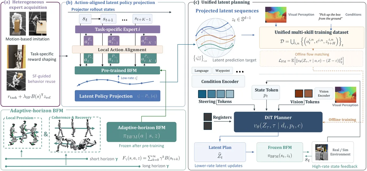
Figure 2: The paper's Fig. 1 overview. (a) Heterogeneous interaction experts acquired through motion imitation, reward shaping, or successor-feature-guided behavior reuse. (b) LPP maps their short-horizon control responses into a frozen AH-BFM; closed-loop rollouts produce executable latent trajectories. (c) Those trajectories train a unified perceptive planner entirely offline, with language or waypoint conditions encoded as steering tokens and a DiT predicting future latent trajectories; at deployment the planner replans from onboard observations while the frozen BFM supplies high-frequency feedback.

Experimental Results

Simulation evaluation runs in IsaacSim with 128 variations per task: box size and initial placement for pickup, door geometry for opening, object identity for grasping. The variation ranges reported in Appendix Tab. X are wide. Boxes use a 20x30x40 cm base independently scaled by $s_x,s_y\in[0.5,1.5]$ and $s_z\in[0.5,1.0]$, spanning 10x15x20 cm to 30x45x40 cm, placed either on the ground or on supports 0.25-0.50 m high, with mass sampled from 0.5-1.5 kg. Doors range 0.8-1.1 m wide and 1.9-2.2 m high, with handle height 0.85-0.95 m above ground and lateral inset 0.08-0.15 m. Grasping evaluates 128 distinct object instances with four takes each — 512 episodes total — selected by teacher-feasibility screening from 685 object instances and 2,991 usable demonstrations. The "with approach" setting initializes the humanoid roughly 0.5-1.5 m from the interaction target and requires it to walk in first; "without approach" starts it directly in front of the target. Success requires the box to be lifted at least 0.3 m and held for at least 1 s, the grasped object lifted at least 0.1 m and held for 1 s, and for door opening the door must be opened and the humanoid must pass through the doorway. Reported plus-minus values come from repeated evaluations under different random seeds.

The main table is organized into three blocks, and reading it correctly depends on keeping them separate: task-specific policies and their projections answer Q1 (how faithfully do experts project), reference-prompted execution answers which representation works at all, and perceptive planning answers Q2 (can one planner learn them jointly). All figures in percent, with Mean computed from the "with approach" columns:

Method	Pickup w/ appr.	Pickup w/o appr.	Door w/ appr.	Door w/o appr.	Grasp Object	Mean
Task-specific policies
Expert Policy†	100.0 ± 0.0	90.8 ± 0.5	89.3 ± 0.2	97.9 ± 0.8	97.0 ± 0.8	95.4
LPP w/ SONIC†	0.0 ± 0.0	0.0 ± 0.0	83.1 ± 0.7	88.1 ± 0.6	5.1 ± 0.7	29.4
LPP w/ Fixed-$\gamma$ BFM†	75.4 ± 0.2	80.2 ± 1.3	61.8 ± 1.9	72.4 ± 0.7	69.3 ± 1.2	68.8
LPP w/ AH-BFM†	81.9 ± 0.9	87.4 ± 2.4	83.5 ± 1.8	97.3 ± 0.4	52.9 ± 2.1	72.8
Reference-prompted execution
SONIC	0.0 ± 0.0	0.0 ± 0.0	0.4 ± 0.0	3.1 ± 0.0	12.1 ± 0.0	4.2
FALCON	0.0 ± 0.0	0.0 ± 0.0	0.4 ± 0.0	2.7 ± 0.0	11.9 ± 0.3	4.1
$B(s)$ Tracking	0.0 ± 0.0	0.0 ± 0.0	0.4 ± 0.0	5.6 ± 0.5	13.9 ± 0.5	4.8
LPP Replay	11.2 ± 0.8	17.7 ± 1.2	12.2 ± 0.9	49.5 ± 0.6	11.3 ± 1.1	11.6
Perceptive planning
OmniContact∗	29.9 ± 0.2	49.6 ± 0.0	–	–	–	–
LessMimic	38.3 ± 0.0	28.5 ± 0.0	–	–	–	–
Action Planner	0.0 ± 0.0	0.0 ± 0.0	0.0 ± 0.0	0.0 ± 0.0	0.0 ± 0.0	0.0
Kinematic Planner	0.0 ± 0.0	0.0 ± 0.0	0.0 ± 0.0	0.0 ± 0.0	10.6 ± 0.5	3.5
FIBER (ours)	42.1 ± 0.6	44.1 ± 1.0	53.5 ± 4.8	51.2 ± 1.0	30.3 ± 2.3	42.0

Table 1: The paper's Tab. I, simulation success rates in percent. ^† denotes a task-specific policy and ^∗ denotes access to privileged object states instead of egocentric observations. Mean is computed from the "w/ appr." results.

The answer to Q1 is task-dependent, and the paper does not smooth that over. LPP with AH-BFM preserves box pickup from 100.0% to 81.9% with approach and from 90.8% to 87.4% without — essentially lossless in the interaction regime — and door opening from 89.3% to 83.5%, with the no-approach figure barely moving at all (97.9% to 97.3%). Fine-grained grasping is a different story, dropping from 97.0% to 52.9%. There is a structural explanation available: grasping depends on high-precision finger coordination, and hand-joint targets are produced by a separate regression branch that is neither constrained to the sphere nor covered by the 29-dimensional normalized action-alignment loss, so projection fidelity there is inherently weaker than for the body. The LPP w/ SONIC row is equally informative in the other direction — swapping the BFM for SONIC collapses pickup to 0.0% and leaves grasping at 5.1% — which shows that the quality of the executable latent space sets the ceiling on projection. Not every unified controller can serve as the substrate.

The representation comparison is about as clean as these ablations get. $B(s)$ Tracking and LPP Replay are derived from the same successful expert trajectories; the former identifies behavior from the expert state trajectory while the latter identifies latent commands from the expert's action responses. The gap on pickup and door opening — 0.0% and 0.4% versus 81.9% and 83.5% — is not a margin, it is a category difference. The paper's conclusion is correspondingly strong: behavioral-state matching alone does not retain interaction-critical feedback. At the other extreme the Action Planner fails on every task, showing that low-rate action planning cannot substitute for the high-frequency state feedback the frozen BFM provides. With both extremes excluded on the same data, the middle path — action-aligned latents executed by a high-rate frozen controller — is the only configuration that survives.

The answer to Q2 lives in the jump from 11.6% to 42.0%. LPP Replay open-loops the projected latent trajectories; FIBER closes the loop with perceptive replanning. Same representation, same BFM, same experts — adding perception-conditioned replanning raises mean success by a factor of 3.6. The authors draw a conclusion worth keeping: high-frequency BFM feedback alone is insufficient, and task-level latent replanning remains important. In the same perceptive-planning block, the Kinematic Planner reaches only 3.5% mean (its single nonzero entry being 10.6% on grasping) and the Action Planner is uniformly zero, while OmniContact — which uses privileged object states — reaches 29.9% on pickup and LessMimic 38.3%. FIBER's 42.1% is obtained from onboard egocentric depth alone, which matters more than the headline number. The paper is also candid about a missing baseline: on-policy multi-expert distillation is not reported, because the experts use different environments, observation spaces and codebases and therefore do not share the online rollout interface joint distillation requires.

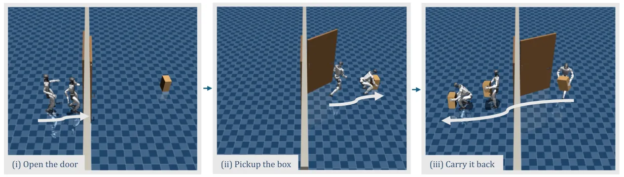
Figure 3: The paper's Fig. 2, skill chaining in simulation. Within a single rollout the same policy sequentially opens the door in (i), picks up the box in (ii), and carries it back through the doorway in (iii), demonstrating closed-loop chaining of multiple interaction skills under changing high-level commands.

Real-world evaluation (Q2 and Q3) deploys the unified planner on a Unitree G1 with an onboard RealSense depth camera. All experts, latent projectors and the unified planner are trained entirely in simulation; nothing is fine-tuned on hardware.

Method	Pickup Box	Open Door	Grasp Object	Mean
FIBER (unified planner, Unitree G1)	6/10	4/10	2/10	40%

Table 2: The paper's Tab. II, real-world success rates of the unified FIBER planner on the Unitree G1. The near-coincidence of 42.0% in simulation and 40% on hardware is the most direct sim-to-real evidence in the paper.

Grasping degrades further on hardware (2/10), which the authors attribute to inaccurate depth estimates for small objects compounding the fine-grained control difficulty — the same weakness that shows up as 30.3% in simulation, seen from two angles. The paper argues, reasonably, that the most informative real-world results are not the success counts but the behaviors in Fig. 3. When the box becomes unstable the robot briefly lifts it and repositions its hands underneath for more secure support. When disturbed while carrying, it stabilizes on its knees, recovers, and continues following waypoint commands. Facing a heavy door, it leans its whole body into the interaction to generate enough pushing force. None of these are explicitly modeled by the planner; they emerge from the fact that planned latents remain grounded in closed-loop physical responses, which is exactly the property the representation was chosen for.

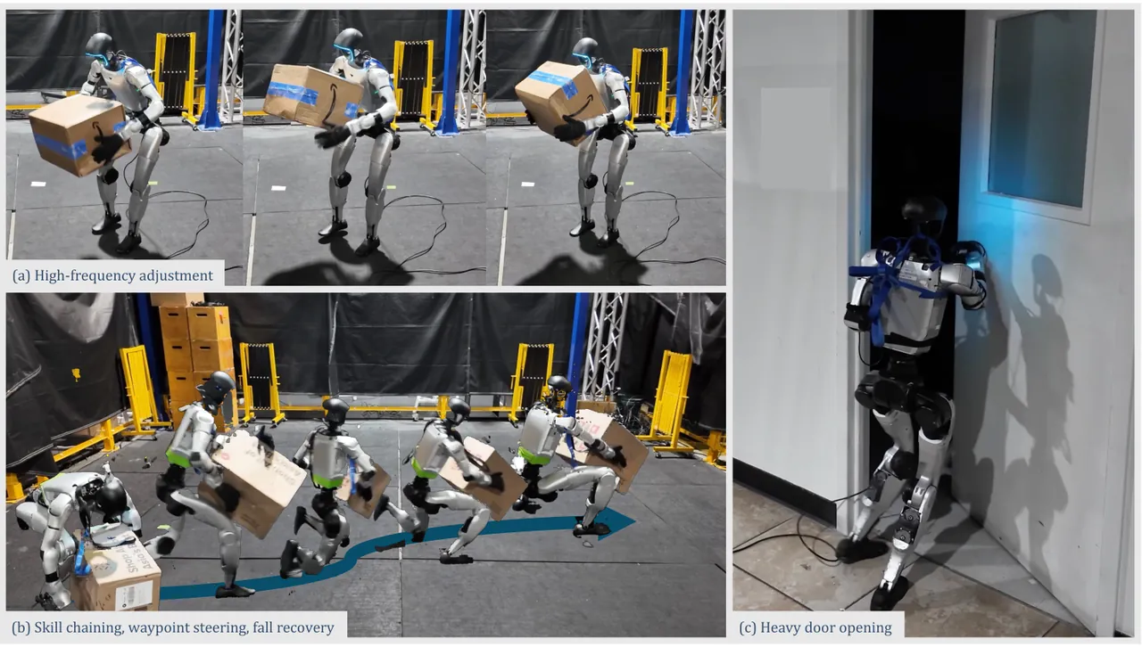
Figure 4: The paper's Fig. 3, qualitative real-world behaviors. (a) High-frequency closed-loop adjustment during box carrying as the robot repositions its hands underneath an unstable grasp. (b) Post-pickup waypoint following, stumbling, knee stabilization, recovery and continuation — interaction-preserving skill chaining, steering and recovery in one sequence. (c) Whole-body leaning into a heavy door to generate sufficient contact force.

The Q4 ablations come in two parts. For the temporal horizon, the paper evaluates AH-BFM on 100STYLE with two complementary metrics: Joint-MAE measures instantaneous motion-tracking accuracy, while BE-EMD measures how well a fixed latent command preserves a reference behavior over increasing embedding horizons — for each reference clip a single latent is inferred through LPP, the BFM is rolled out under that fixed command, and the discrepancy from the reference is measured.

Method	Joint-MAE ↓	BE-EMD 0.2 s ↓	BE-EMD 0.5 s ↓	BE-EMD 1 s ↓	BE-EMD 2 s ↓
SONIC	0.1315	–	–	–	–
BFM $\gamma_{0.8}$	0.1107	0.038	0.200	0.495	0.792
BFM $\gamma_{0.98}$	0.1327	0.048	0.213	0.451	0.601
AH-BFM	0.1020	0.049	0.195	0.422	0.590

Table 3: The paper's Tab. III, ablation of multi-horizon BFM tracking and behavior-embedding performance on 100STYLE. Bold marks the best value in each column.

This table lays the trade-off out without argument. The short-horizon model $\gamma=0.8$ wins BE-EMD at 0.2 s (0.038) but degrades badly at 2 s (0.792). The long-horizon model $\gamma=0.98$ is better at long horizons (0.601 at 2 s) yet has the worst Joint-MAE of all four rows at 0.1327 — worse even than SONIC's 0.1315. AH-BFM attains the lowest Joint-MAE at 0.1020 (8% better than $\gamma=0.8$ and 23% better than $\gamma=0.98$) and the lowest BE-EMD at 0.5, 1 and 2 s, conceding only the 0.2 s column at 0.049 versus 0.038. Adaptive multi-$\gamma$ learning therefore captures most of what each fixed horizon is good at, paying for it only at the shortest horizon. The advantage propagates to interaction projection: replacing the fixed-$\gamma$ BFM ($\gamma=0.98$) with AH-BFM in Tab. I raises mean LPP success from 68.8% to 72.8%, with substantial gains on box pickup (75.4 to 81.9) and door opening (61.8 to 83.5).

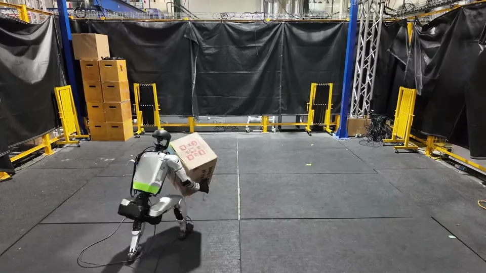
Figure 5: Project-page material showing one product of SF-guided behavior reuse: the same carrying interaction composed with crouch-walking, where the controller must maintain support of the box while realizing a substantially different whole-body configuration. Compositions of this kind require no new motion reference and no new expert — only a different requested native latent $z^{N}$.

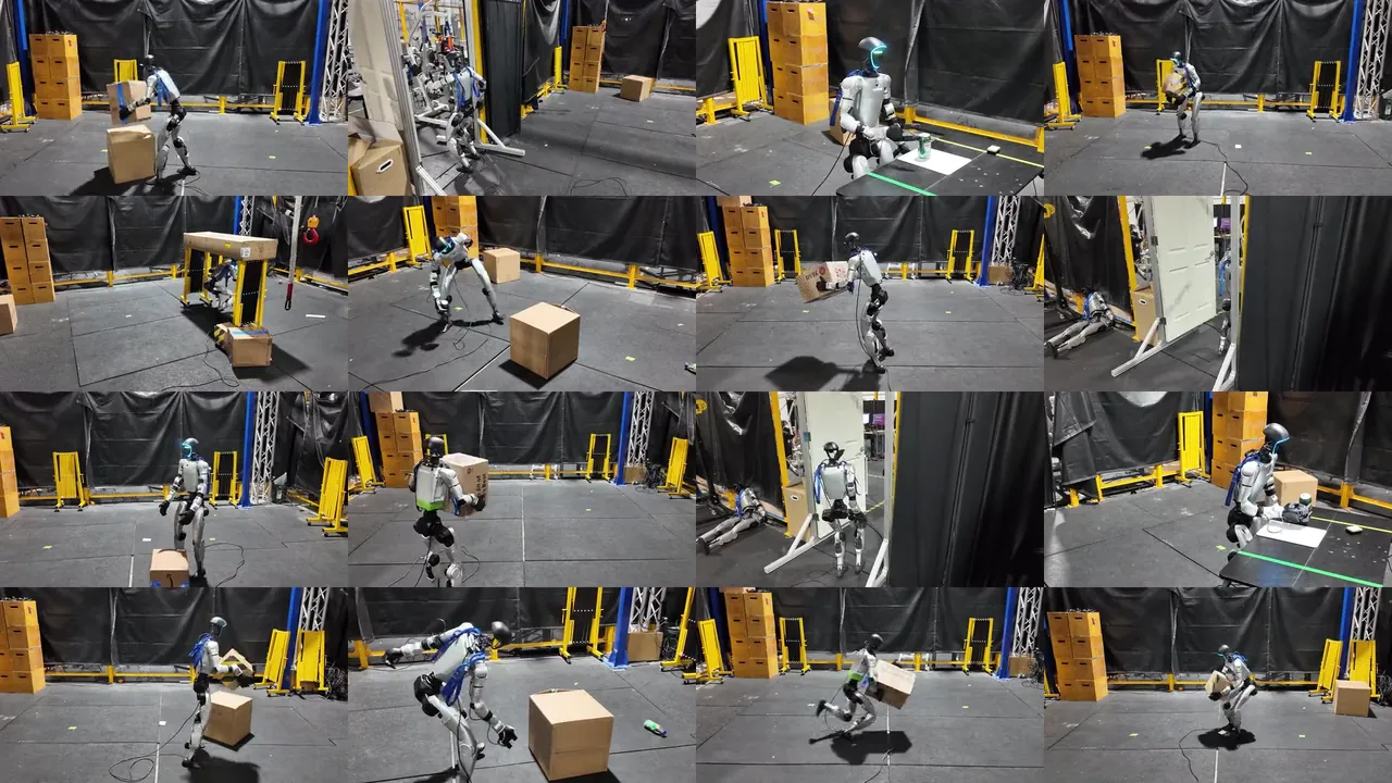
Figure 6: The project page's capability grid — one unified planner covering three heterogeneous interactions (box pickup, door opening, object grasping), composed with native whole-body behaviors such as walking, crouch-walking and kneeling, and steerable through language or waypoint conditions.

Limitations

First, and stated by the authors: the underlying BFM caps the whole system. The conclusion names two directions explicitly — extending the BFM toward more dynamic whole-body behaviors such as stair traversal, and incorporating richer visual and tactile feedback together with online latent adaptation to support more diverse contact conditions and continual integration of new skills. Neither is decorative. The AH-BFM latent space is trained offline and frozen throughout; however strong the planner is, it can only compose within the behavior set that space spans. Dynamics absent from the latent space are dynamics FIBER cannot invoke, and no amount of planning compensates for that.

Second, fine manipulation is a clear weakness, and it degrades at two separate stages. On grasping, the chain runs expert 97.0% → LPP 52.9% → unified planner 30.3%, and only 2/10 on hardware. That three-step decay says the problem is not confined to the planner. Hand-joint targets bypass the sphere and the 29-dimensional action-alignment loss through a separate regression head, so projection fidelity is structurally weaker there; on top of that sits monocular metric depth at 144x256 with a 0.12-3.0 m valid range, whose error on small objects is significant relative to the tolerances grasping demands. Fine manipulation is the least robust link in the entire pipeline.

Third, absolute performance still trails the specialists by 53 points, and the strongest competing baseline is missing. Beating 11.6% and 3.5% by an order of magnitude establishes the representation choice; trailing the task-specific experts at 95.4% by 53.4 points means this is a workable general interface rather than a deployable replacement for specialists — pickup falls 100.0 to 42.1 and grasping 97.0 to 30.3. More consequential for interpretation is the absent on-policy multi-expert distillation comparison, excused on the grounds that the experts do not share an online rollout interface. That is precisely the design FIBER's decoupled setting competes against, so the reader cannot tell whether 42.0% is the necessary price of decoupling or the price of this particular projection-plus-offline-planning implementation.

Fourth, the coverage boundary of the offline supervision is never quantified. The planner is trained entirely offline on 20K projected closed-loop episodes per skill. DAgger-style aggregation exposes the projector to corrective states, but the planner still only sees the state distribution of the projected policies. When deployment encounters scenes outside that distribution — novel objects, lighting, terrain — the system has no online adaptation mechanism, which the authors themselves list as future work. No quantitative out-of-distribution generalization result is reported, and ten real-world trials per task is a small sample on which to rest a sim-to-real claim.

Conclusion and Outlook

FIBER's real contribution is not a new network but a defensible answer to the question of what belongs between high-level planning and whole-body control: an executable, state-dependent behavioral latent command. Kinematic targets discard the control response; low-level actions discard high-frequency feedback; a BFM latent keeps both, because it indexes a policy rather than a trajectory. Around that judgment the paper supplies three pieces of supporting engineering, each addressing a specific failure mode: action alignment ($\mathcal{L}_{\mathrm{act}}$) on physical joint targets rather than state or behavior matching, spherical semantic anchoring ($\mathcal{L}_{\mathrm{sem}}$) to resolve action-equivalent ambiguity, and multi-$\gamma$ FB learning (AH-BFM) so one latent space satisfies both the short-horizon precision projection needs and the long-horizon coherence planning needs.

The engineering value of the decoupled setting may outlast the performance numbers. Experts can be trained in different codebases with different observations and rewards; once projected, the original experts are discarded and the planner trains from offline latent trajectories alone. Adding a new skill therefore does not require standing up a joint training pipeline or making separate teams' simulation environments mutually compatible. SF-guided behavior reuse compounds this by reducing the cost of an interaction-times-behavior combination from "one motion reference per combination" to "swap the requested native latent $z^N$." For a robot skill library that has to keep growing, that additivity is worth more than any single success rate.

Read against the evidence, the current state is "interface validated, precision outstanding." The 42.0% versus 3.5% comparison shows the representation choice is right; 42.0% versus 95.4% shows it cannot yet replace specialists. The three most informative next steps are adding online latent adaptation (already flagged by the authors as future work), bringing dexterous hands inside the same action-alignment objective instead of a bypass regression head, and supplying a genuine on-policy multi-expert distillation comparison. If those hold up, "frozen BFM latent space as a general behavioral bus" is a plausible standard way to organize humanoid skill libraries.

Golden Quotes