PAPER DEEP DIVE
ImprovedVBGS: Real-time Continual Variational Bayes Gaussian Splatting
On-the-fly reconstruction is a key requirement for many applications in robotics and autonomous navigation. Variational Bayes Gaussian Splatting (VBGS) enables continual learning without replay buffers using Coordinate Ascent Variational Inference (CAVI), but its per-frame iterations over all observed points make it too slow for real-time use with strict memory and latency requirements. We present ImprovedVBGS, an accelerated framework for on-the-fly continual reconstruction. This is achieved primarily through (i) spatially truncated variational inference, and (ii) improved reassignment that uses forwarding, truncation and eliminates wasteful dynamic recompilation. On the NeRF synthetic dataset, we reduce mean per-frame latency from ~84.0 s to ~0.050 s on an RTX 3070 Ti, a 1680x speed-up while maintaining reconstruction quality.
ImprovedVBGS: Real-time Continual Variational Bayes Gaussian Splatting
Author: Damani Mguni-Coker (Independent Researcher) | arXiv: 2607.15542v1 | Code: github.com/damanimc/ImprovedVBGS
One-Sentence Summary
ImprovedVBGS achieves a 1680× speedup (84.0s → 0.050s per frame on RTX 3070 Ti) over VBGS through spatially truncated variational inference and improved reassignment (forwarding + truncation + eliminating dynamic recompilation), while maintaining reconstruction quality for real-time continual 3D reconstruction on consumer hardware.
Background and Motivation
On-the-fly reconstruction is critical for robotics and autonomous navigation. 3D Gaussian Splatting (3DGS) represents scenes as collections of 3D Gaussians parameterized by mean $\mu \in \mathbb{R}^3$, covariance $\Sigma$, opacity $\alpha$, and spherical harmonic coefficients.
In continual learning, data arrives sequentially and gradient methods suffer catastrophic forgetting. Replay buffers mitigate this but increase memory/compute with the number of observed views, unsuitable for resource-constrained scenarios.
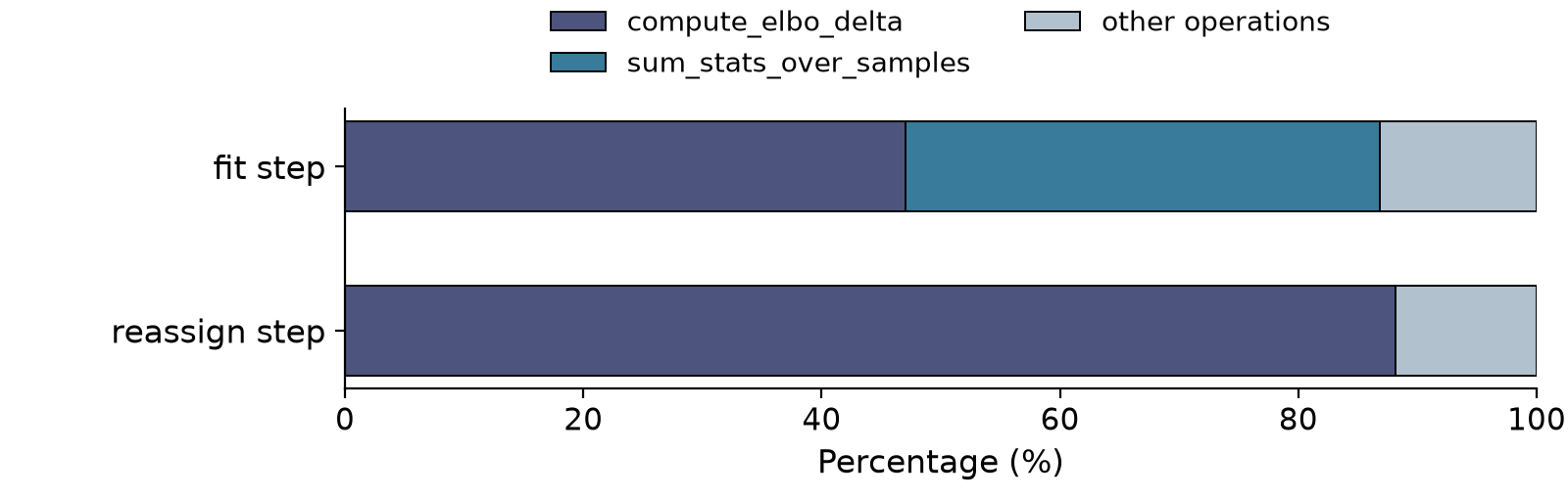
Figure 1: VBGS generative model. Each point's position $s$ and color $c$ are generated by latent component assignment $z \sim \mathrm{Cat}(\pi)$.
VBGS formulates the problem as variational inference over a probabilistic mixture model with conjugate priors (Normal-Inverse-Wishart for position/color, Dirichlet for weights). Updates are order-invariant and accumulate sufficient statistics, making VBGS inherently immune to catastrophic forgetting without replay buffers. However, each update evaluates responsibilities for all $n$ points across all components ($O(nK)$), growing linearly with scene size. Prior work [11] reduced training from 234 to 61 minutes via kernel fusion and mixed precision, but still processes all observed points, leaving per-frame latency far too high for real-time use.
Method Details
1. Fused Sufficient Statistics and Mixed-Precision Search
Reproduces [11]'s kernel fusion (eliminating large intermediate tensors) and automatic mixed-precision search. However, mixed precision provides no benefit once spatial truncation is applied.
2. Spatially Truncated Variational E-step
Variational inference estimates the posterior by maximizing the ELBO:
$$\text{ELBO}=\sum_{n=1}^{N}\big(\mathbb{E}_{q}[\log p(s_{n}|z_{n},\mu_{s},\Sigma_{s})]+\mathbb{E}_{q}[\log p(c_{n}|z_{n},\mu_{c},\Sigma_{c})]+\mathbb{E}_{q}[\log p(z_{n}|\pi)]\big)$$The E-step computes component assignment expectations. Log-responsibilities combine spatial likelihood, color likelihood, and mixture weight:
$$\log\gamma_{n,k}\propto\underbrace{\mathbb{E}_{q(\mu_{k,s},\Sigma_{k,s})}[\log p(s_{n}|\mu_{k,s},\Sigma_{k,s})]}_{\text{spatial likelihood}}+\underbrace{\mathbb{E}_{q(\mu_{k,c},\Sigma_{k,c})}[\log p(c_{n}|\mu_{k,c},\Sigma_{k,c})]}_{\text{color likelihood}}+\underbrace{\mathbb{E}_{q(\pi)}[\log\pi_{k}]}_{\text{mixture weight}}$$Key insight: spatial likelihood concentrates mass on nearby means. Per frame, a KD-tree $T$ is built on spatial means, and $C$ nearest-neighbor components are queried per point, evaluating log-scores only on that subset:
$$R_{n}=\mathrm{softmax}(\log\hat{\gamma}_{n}), \quad \mathrm{ELBO}_{n}=\mathrm{logsumexp}(\log\hat{\gamma}_{n})$$This reduces complexity from $O(nK)$ to $O(nC)$ where $C \ll K$ (e.g., $C=4$).
The complexity reduction can be formalized. The original E-step evaluates all $K$ components:
$$T_{\text{dense}} = O(n \cdot K)$$After truncation, only $C$ nearest neighbors are evaluated:
$$T_{\text{trunc}} = O(n \cdot C + n \cdot \log K)$$where $n \log K$ is the KD-tree query cost. With $K = 10^5$, $C = 4$, the speedup ratio is approximately $K / (C + \log K) \approx 10^4 / (4 + 17) \approx 476\times$.
3. Improved Reassignment
Reassignment relocates unused components to poorly modeled regions. Each component $k$ has Dirichlet weight $\alpha_k$; unassigned components decay to the prior floor. Per step, the lowest 5% $\alpha_k$ components are moved to lowest-ELBO regions. Per-point ELBO:
$$\text{ELBO}_{n}=\log{\sum_{k=1}^{K}\exp(\log\hat{\gamma}_{n,k})}$$Truncated Reassignment: ELBO values from the E-step are reused directly. Reassignment Forwarding: ELBO values forwarded from the fit step (reordering steps), trading small PSNR drop for lower latency. Static Tensor Padding: $n_{\mathrm{reassign}}$ varies per frame causing JAX recompilation; padding to fixed compile-time shape $n_{\max}=\lfloor f \cdot N \rfloor$ eliminates this.
flowchart TD
    A["Input: RGB-D frame with depth"] --> B["Build KD-tree on spatial means"]
    B --> C["Truncated E-step: query C nearest neighbors per point"]
    C --> D["Compute truncated responsibilities R_n and ELBO_n"]
    D --> E["M-step: update posterior parameters
(sufficient statistics accumulation)"]
    E --> F["Reassignment: truncated ELBO + forwarding
static tensor padding"]
    F --> G["Output: updated 3D Gaussian scene"]
    C -.->|"ELBO reuse"| F
Experimental Results
Evaluated on RTX 3070 Ti (8GB VRAM), significantly more constrained than the A5000 (24GB). All 8 NeRF Synthetic scenes, 200 training + 100 validation frames, $N=10^5$ components, random initialization.
| Scene | Latency (s/frame) | PSNR (dB) |
|---|---|---|
| chair | 0.128 | 21.68±0.62 |
| drums | 0.132 | 18.48±0.44 |
| ficus | 0.117 | 21.06±0.69 |
| hotdog | 0.143 | 23.40±0.74 |
| lego | 0.136 | 21.54±0.69 |
| materials | 0.133 | 20.51±1.41 |
| mic | 0.117 | 23.43±0.55 |
| ship | 0.159 | 21.30±0.77 |
| Mean | 0.133 | 21.42±0.74 |
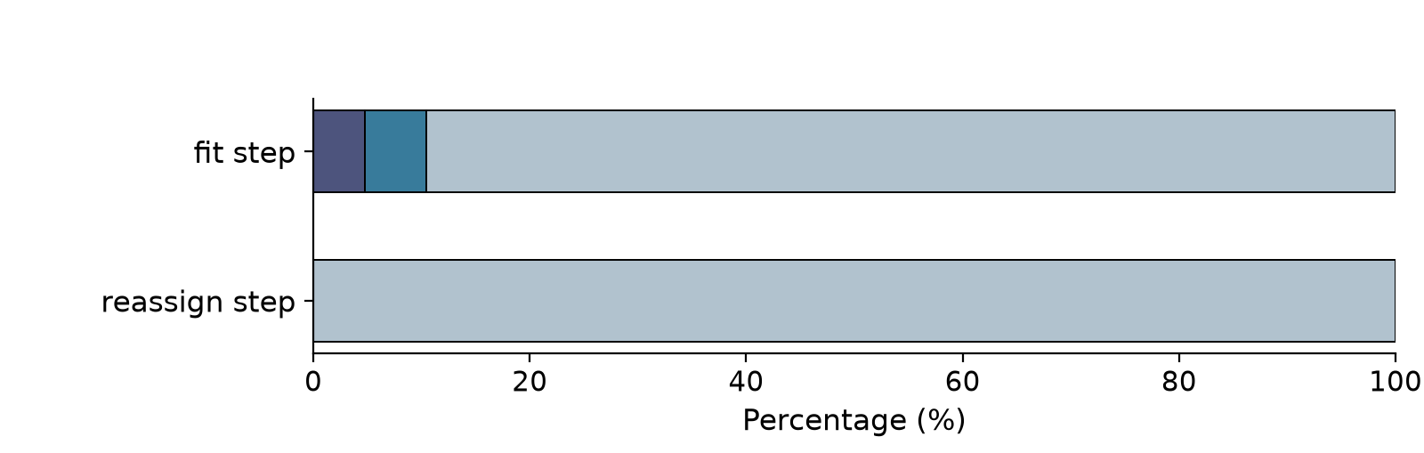
Figure 2: Latency composition on Lego. Baseline VBGS fit step dominated by compute_elbo_delta (28.8s/frame, 47%) and sum_stats (24.3s/frame, 40%); in ImprovedVBGS each drops to ~5%.
Ablation Study (Lego)
| Configuration | Batch Size | Latency (s/frame) | PSNR (dB) |
|---|---|---|---|
| Baseline VBGS | 100 | 84.0 | 20.65±0.92 |
| + Fused Stats | 100 | 41.0 | 20.65±0.92 |
| + Truncated E-step | 100 | 3.39 | 20.64±0.92 |
| + Large Batch | 250k | 0.050 | 20.64±0.92 |
| + Reassignment | 250k | 18.1 | 21.48±0.72 |
| + Truncated Reassignment | 250k | 0.373 | 21.56±0.69 |
| + Static Tensor Padding | 250k | 0.131 | 21.57±0.69 |
| + Reassign Forwarding | 250k | 0.107 | 21.37±0.70 |
1680× speedup without reassignment (84.0→0.050s), 785× with reassignment forwarding (84.0→0.107s). Reassignment improves PSNR from 20.64 to 21.48+; truncated reassignment further reduces to 0.373s with slightly higher PSNR.
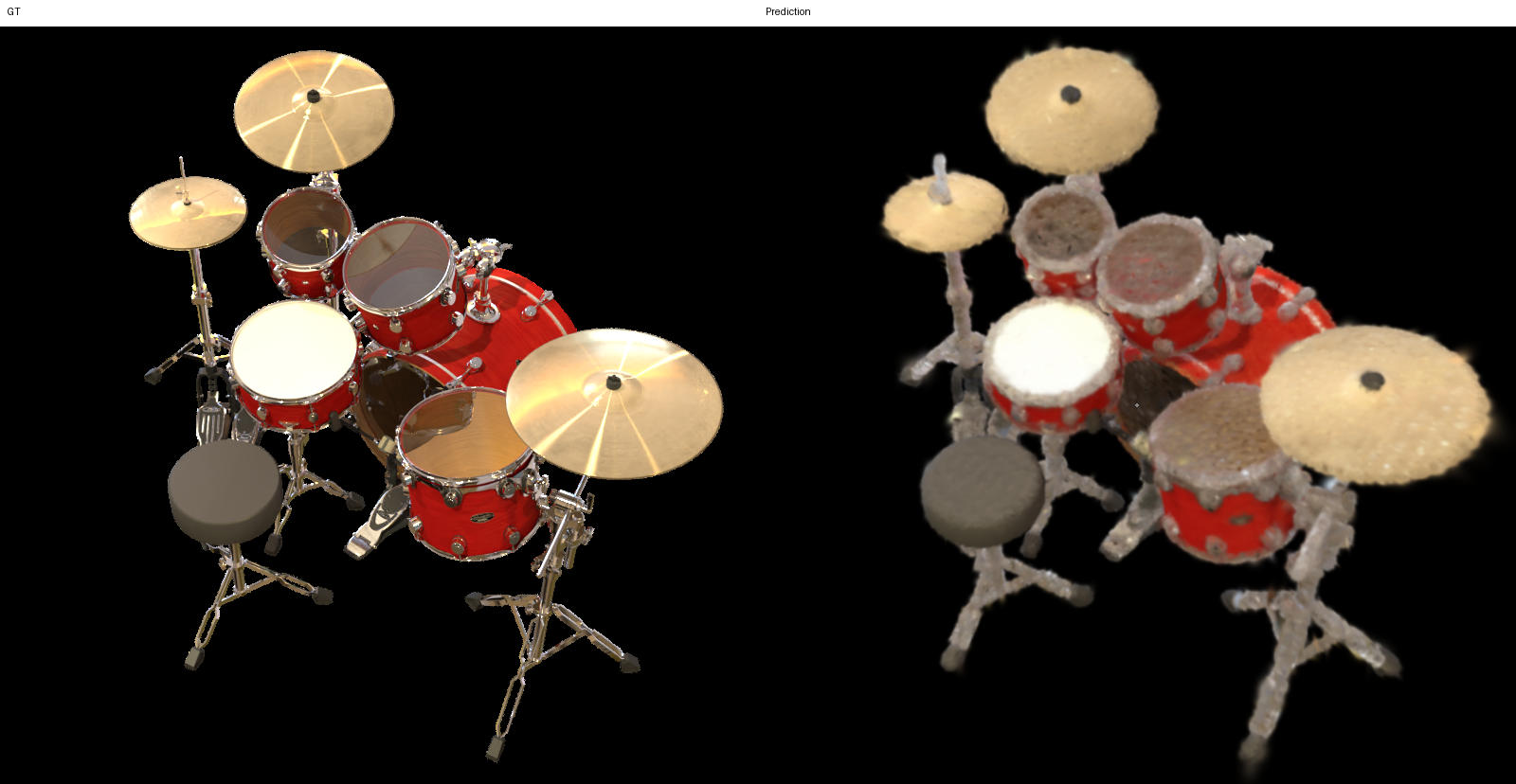
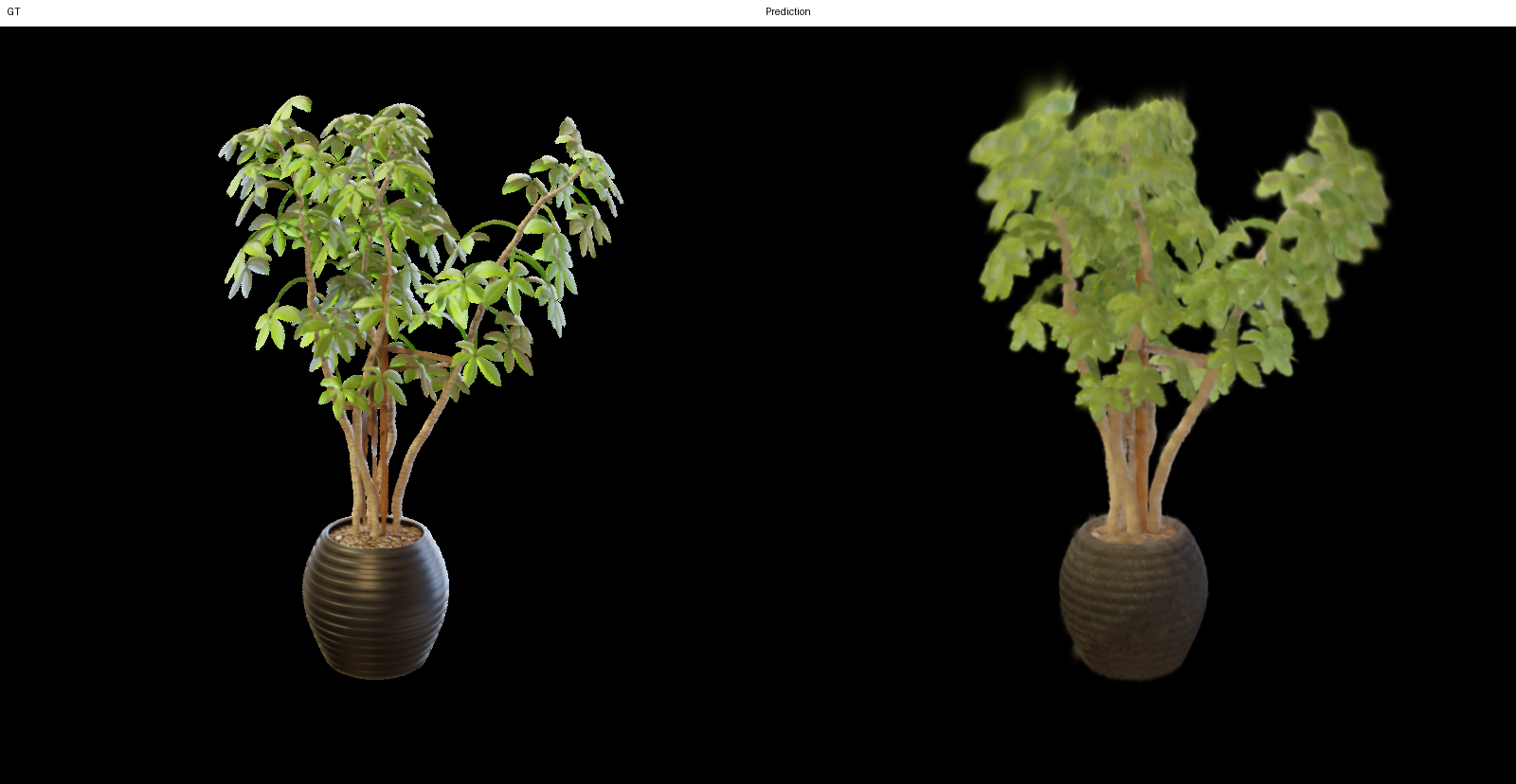
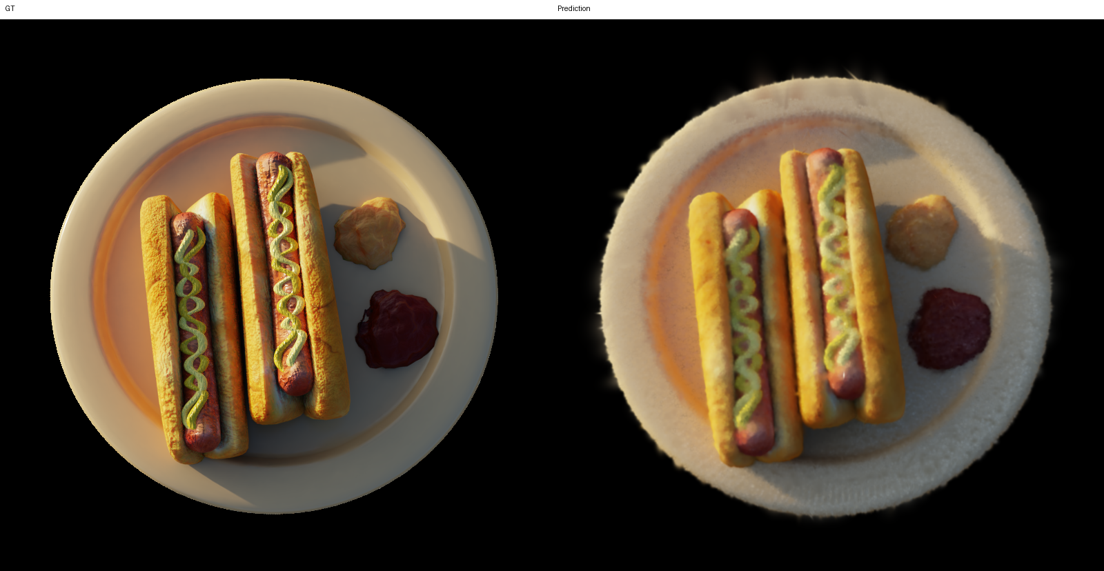
Figure 4: Additional scene reconstruction visualization.
Latency Analysis Details
The baseline VBGS fit step is dominated by two operations: compute_elbo_delta at 28.8s/frame (47%) and sum_stats_over_samples at 24.3s/frame (40%), with the rest at only 8.1s/frame. In ImprovedVBGS, these drop to 3.1ms/frame (4.8%) and 3.7ms/frame (5.6%) respectively, with other operations at 58.4ms/frame.
In the reassignment step, baseline compute_elbo_delta accounts for 22.7s/frame (88%). ImprovedVBGS completely removes this recomputation, retaining only 107ms/frame for other operations. This demonstrates that truncated E-step not only accelerates the fit step but also eliminates the main bottleneck of the reassignment step through ELBO reuse.
Batch Size and Memory Optimization
Baseline VBGS with $N=10^5$ components can only use a batch size of 100 to avoid OOM errors. After fused statistics and truncated E-step optimizations, the batch size increases to 250,000, fully exploiting GPU parallelism. This increase is critical for latency reduction — from 3.39s/frame with truncated E-step to 0.050s/frame, a 67.8× improvement primarily from large-batch parallelization.
Comparison with VBGS Ecosystem
VBGS [10] first introduced variational inference to Gaussian Splatting, enabling replay-free continual learning, but its 84s/frame latency made real-time use impossible. Zaino et al. [11] reduced training from 234 to 61 minutes and memory from 9.44GB to 1.1GB via kernel fusion and mixed precision, enabling edge deployment on Jetson Orin Nano. ImprovedVBGS further reduces per-frame latency from seconds to milliseconds, making true on-the-fly reconstruction feasible. The three form a progressive optimization chain: VBGS established the theoretical foundation → [11] achieved edge feasibility → ImprovedVBGS achieved real-time performance.
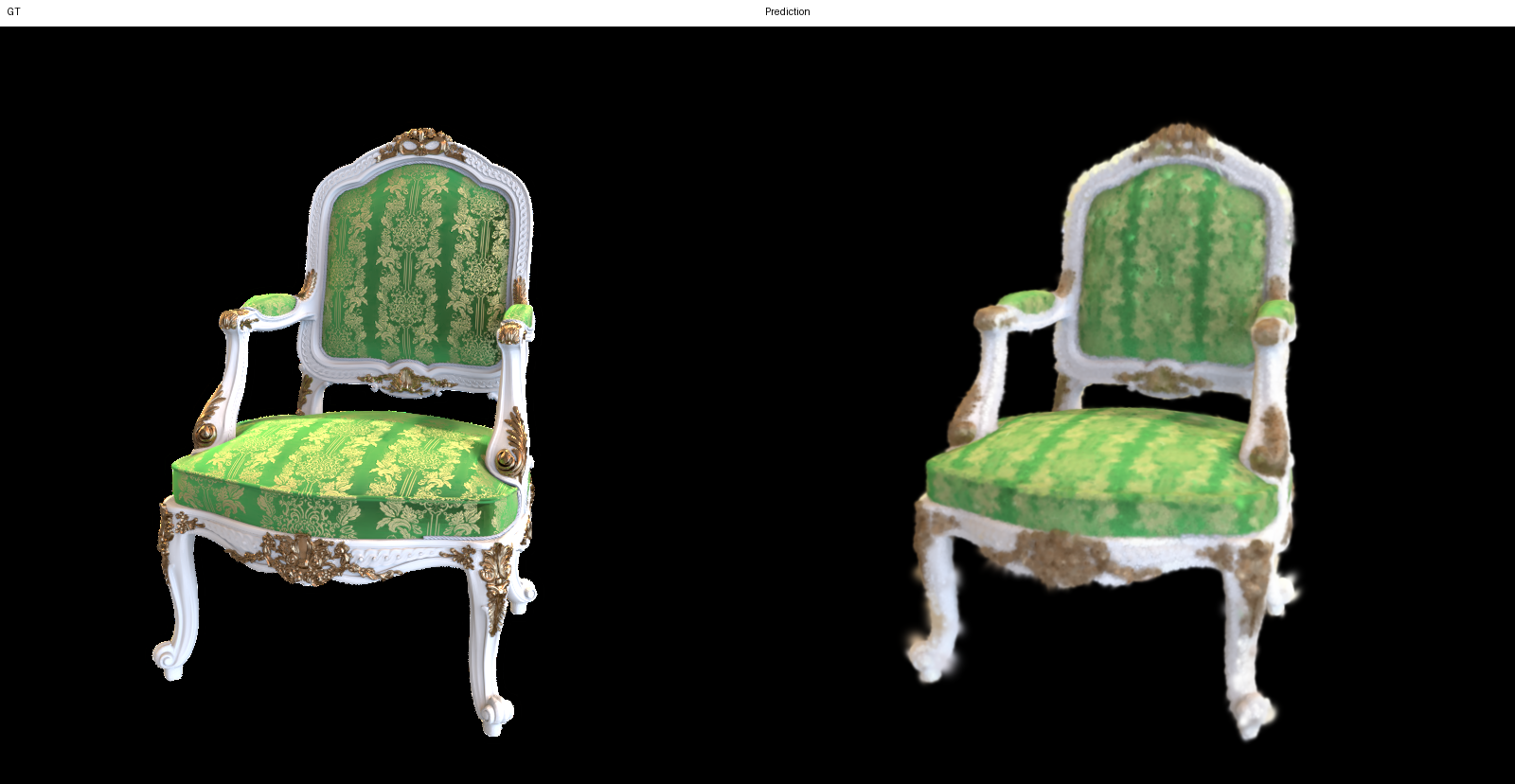
Figure 3: NeRF Synthetic dataset reconstruction visualization.
Limitations
- Requires depth input (unlike traditional 3DGS using only RGB), limiting applicability.
- Uses over 2× parameters (29 vs 14), does not model view-dependent color via spherical harmonics.
- Evaluated on RTX 3070 Ti, not validated on lower-end edge devices.
- Reassignment forwarding trades a small PSNR drop (~0.2dB) for lower latency.
Conclusion and Outlook
ImprovedVBGS reduces VBGS per-frame latency from 84s to 0.05s via spatially truncated variational E-step (KD-tree nearest-neighbor pruning) and improved reassignment (truncated ELBO reuse + forwarding + static tensor padding), enabling real-time continual 3D reconstruction on consumer hardware while preserving replay-free continual learning. The core contribution reduces E-step complexity from $O(nK)$ to $O(nC)$ and eliminates JAX dynamic recompilation overhead.
Key insight: "Spatial likelihood concentrates mass on nearby means" — this simple observation enables order-of-magnitude acceleration without quality loss, pushing variational Bayes Gaussian Splatting from academic prototype toward real-time deployment.
Deep analysis generated by RobotWorld paper-detail-generator based on full-text reading | arXiv:2607.15542v1