JEPA-Anything: Learning Predictive Models across Different Worlds

Paper Information

Title: JEPA-Anything: Learning Predictive Models across Different Worlds

Authors: Taoyong Cui, Zhongyao Wang, Xinyue Xu, Weiyang Liu, Zhaochen Yu, Yuying Zhang, Qiang Gao, Mengyue Yang, Wanli Ouyang, Pheng Ann Heng, Yingcheng Wu, Zhenfei Yin, and Ling Yang.

Paper: arXiv:2609.20800, submitted on September 17, 2026.

Code status: The public Gen-Verse/JEPA-Anything repository exposes the reusable OPF core, a design validator, a structural recipe, and an artifact manifest. It explicitly does not contain the paper's domain datasets, full training pipelines, or trained model weights, so it supports implementation and geometric auditing rather than one-command reproduction of every reported result.

Background and Motivation

A world model learns an internal state that lets an agent or scientific model anticipate an unobserved, intervened, or future state of a system. The target can be a hidden image region, a patient's future health state, a molecular configuration, or the next state of a physical field. The paper adopts a broad but operational definition: the context and target must belong to the same underlying system and have usable statistical dependence, while the learned state should support readout, repeated transition, or analysis.

Joint-embedding predictive architectures provide the natural starting point. An online encoder summarizes the visible context, an EMA target encoder defines the prediction target, and a predictor maps the context representation into the target representation. Latent-space prediction avoids spending capacity on irrelevant pixel detail, but the standard JEPA formulation still compresses the requested target into one embedding and one prediction pathway.

That monolithic interface creates a capacity-allocation problem. A visual state can combine location, object identity, and transformation. A physical field combines entities, scales, and dynamical modes. A clinical state contains sparse and irregular events. A molecular state contains geometry, velocity, species, and a simulation cell. When all of these structures share one target embedding, high-variance or easily predicted directions can dominate optimization, while weaker but useful structure receives conflicting gradients.

JEPA-Anything addresses this by keeping the domain boundary honest. Each domain supplies its own adapter, context-target sampling rule, encoders, and base loss. Once the context and target states exist, however, the same factorized predictive core is used across domains. The paper therefore treats the problem as one of structuring predictive capacity, not as a claim that radically different observations should share a single encoder or set of weights.

The proposed mechanism is Orthogonal Predictive Factorization, or OPF. It partitions the target state into learned subspaces, assigns a dedicated predictor to each subspace, keeps every coordinate active, and recombines the predictions into a complete state. The resulting interface can be used once for readout, repeatedly for rollout or planning, or retained as a diagnostic coordinate system for scientific analysis.

Required Concepts

Let $d$ be the width of the latent world state, $z_c$ the online context representation, and $z_t$ the target representation produced by the EMA encoder. The target encoder receives no gradient. Its parameters follow an exponential moving average of the online encoder, so the target representation changes gradually while the online encoder learns.

OPF requires a complete factorization: $K r=d$, where $K$ is the number of factors and $r$ is the width of each factor. This is stronger than adding several heads to the same latent vector. It means the factor subspaces form a partition of the full state dimension. Factor indices remain anonymous until evidence from probes, interventions, or external experiments assigns meaning to them.

The method also preserves both analysis and synthesis. Analysis projects a state through $P_k^\top$ into factors. Synthesis applies the Moore-Penrose pseudoinverse of the stacked analysis map to return to the complete state. This explicit route is what separates the work from representation objectives that shape useful features but do not guarantee that the learned components can reconstruct the state they decompose.

Method

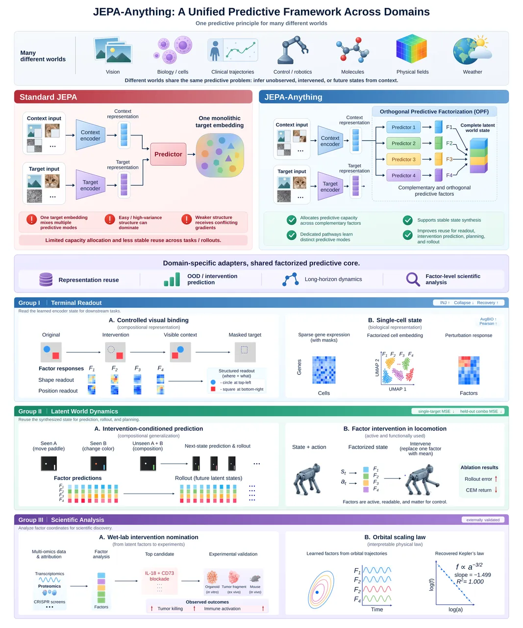
Figure 1: Overview of JEPA-Anything. The upper panel contrasts standard JEPA with orthogonal predictive factorization and state synthesis; the lower panel organizes the three experimental groups.

flowchart LR
    X[Raw observation] --> A[Domain adapter: tokens and descriptors]
    A --> V[Context-target sampler]
    V --> E[Online encoder]
    V --> T[EMA target encoder]
    T --> G[Stop-gradient target state]
    G --> P[K orthogonal projections]
    E --> Q[K dedicated predictors]
    P --> Q
    Q --> U[Predicted factor stack]
    U --> S[Pseudoinverse synthesis]
    S --> Z[Complete latent world state]
    Z --> R[Readout / planner / rollout / analysis]

1. One interface for heterogeneous observations

For domain $\delta$, an adapter $\mathcal{A}_{\delta}$ converts a raw observation $x$ into content tokens $H$ and structural descriptors $S$. The descriptors can encode patch coordinates, timestamps, graph positions, entity identities, or no extra information. A view sampler then selects context indices $C$ and target indices $T$:

$$x\xrightarrow{\mathcal{A}_{\delta}}(H,S)\xrightarrow{\mathcal{V}_{\delta}}(H_C,S_C,T,S_T).$$

The adapter and sampler absorb domain geometry. After that point, the core assumes a common token interface. A ViT can serve images, a Transformer can serve sequences, a GNN can serve graphs, and an MLP can serve fields or tabular records. The shared portion is the online/EMA target scheme, factorized prediction, synthesis, and regularization.

The target encoder is updated as follows:

$$\bar{\theta}\leftarrow m\bar{\theta}+(1-m)\theta,\qquad 0\leq m<1.$$

The online encoder produces $z_c=f_\theta(H_C,S_C)$. The target encoder produces $z_t=f_{\bar{\theta}}(H,S)_t$ for each requested target index. A single target index recovers the usual JEPA case, while multiple indices represent masked regions, spatial locations, time steps, or other structured targets.

2. Orthogonal predictive factorization

OPF learns $K$ projectors $P_k\in\mathbb{R}^{d\times r}$. The target representation is stopped before projection:

$$\widetilde{z}_t=\operatorname{sg}(z_t),\qquad z_t^{(k)}=P_k^\top\widetilde{z}_t,\qquad k=1,\ldots,K.$$

Each factor has its own predictor $q_k$. The predictor receives the shared context state and, when required, a target descriptor:

$$\widehat{z}_t^{(k)}=q_k(z_c,s_t).$$

The descriptor may identify which target location or time is being predicted. If the context already determines the target unambiguously, the predictor can ignore it. The predictors can be independent or share a trunk with factor-specific heads.

The predicted factors are concatenated into $\widehat{u}_t$ and mapped back into the full latent state through the pseudoinverse of the stacked analysis map:

$$\widehat{z}_t=(P^\top)^\dagger\widehat{u}_t\in\mathbb{R}^{d},\qquad P=[P_1,\ldots,P_K].$$

When the projectors are exactly orthogonal, $(P^\top)^\dagger=P$ and the operation reduces to $\widehat{z}_t=\sum_k P_k\widehat{z}_t^{(k)}$. The paper stresses that concatenation alone is not synthesis. The explicit inverse map is the state interface used by downstream decoding, planning, or repeated transition.

For temporal or intervention-conditioned dynamics, let $\xi_t$ denote an action, intervention, or known forcing. The transition becomes:

$$\widehat{u}_{t+1}=\left[q_1(z_t,\xi_t,s_{t+1});\ldots;q_K(z_t,\xi_t,s_{t+1})\right],\qquad \widehat{z}_{t+1}=(P^\top)^\dagger\widehat{u}_{t+1}.$$

Applying this rule repeatedly defines a latent rollout. A planner can score candidate trajectories using a domain reward, while the world model supplies the predicted states.

3. Why prediction, orthogonality, and activity are separate objectives

Each predicted factor is regressed directly to its target instead of using only a cosine or similarity objective:

$$\mathcal{L}_{\mathrm{pred}}=\frac{1}{K|T|r}\sum_{t\in T}\sum_{k=1}^{K}\left\|\widehat{z}_t^{(k)}-z_t^{(k)}\right\|_2^2.$$

Direct regression preserves both direction and magnitude, which matters because the predicted factors must be synthesized into a state. The projectors remain trainable even though the target encoder output is stopped, so prediction, orthogonality, and activity all shape the factor axes.

Prediction alone does not prevent two branches from learning the same direction. The orthogonality objective constrains both within-projector and cross-projector Gram matrices:

$$\mathcal{L}_{\mathrm{orth}}=\sum_{k=1}^{K}\left\|P_k^\top P_k-I_r\right\|_F^2+\sum_{1\leq i<j\leq K}\left\|P_i^\top P_j\right\|_F^2.$$

The first term discourages a degenerate basis inside one factor. The second penalizes overlap between different factor subspaces. In the exact zero-penalty limit, the subspaces form an orthogonal direct sum and preserve the norm of the target state:

$$\left\|P^\top z\right\|_2^2=\sum_{k=1}^{K}\left\|P_k^\top z\right\|_2^2=\left\|z\right\|_2^2,\qquad z=\sum_{k=1}^{K}P_kP_k^\top z.$$

With exact factor coordinates, prediction error $e$ satisfies $\|\widehat{z}-z\|_2=\|e\|_2$, and the stacked projector has condition number $\kappa_2(P)=1$. Without cross-factor orthogonality, repeated or nearly repeated directions can make the map rank deficient or numerically unstable. The appendix extends this intuition to approximately orthogonal maps and shows that the orthogonality residual controls error amplification.

Orthogonal directions can still be inactive. A coordinate may occupy its own subspace but remain almost constant across samples. OPF therefore applies a standard-deviation hinge to every target coordinate and a separate variance term to the online encoder:

$$\mathcal{L}_{\mathrm{fac}}=\frac{1}{Kr}\sum_{k=1}^{K}\sum_{j=1}^{r}\max(0,\gamma_{\mathrm{fac}}-\sigma_{k,j}^{\mathrm{fac}}),\qquad \mathcal{L}_{\mathrm{enc}}=\frac{1}{d}\sum_{j=1}^{d}\max(0,\gamma_{\mathrm{enc}}-\sigma_j^{\mathrm{enc}}).$$

The first term shapes the projectors on stopped-gradient targets. The second sends an anti-collapse signal directly to the online representation. The composite training loss is:

$$\mathcal{L}_{\mathrm{OPF}}=\mathcal{L}_{\mathrm{pred}}+\lambda_{\mathrm{orth}}\mathcal{L}_{\mathrm{orth}}+\lambda_{\mathrm{fac}}\mathcal{L}_{\mathrm{fac}}+\lambda_{\mathrm{enc}}\mathcal{L}_{\mathrm{enc}},\qquad \mathcal{L}_{\mathrm{train}}^{(\delta)}=\mathcal{L}_{\mathrm{base}}^{(\delta)}+\mathcal{L}_{\mathrm{OPF}}.$$

JEPA-Anything therefore adds a shared core to an existing domain objective rather than replacing it. The dimensions and weights can change by domain, but the functional form of the objective remains the same.

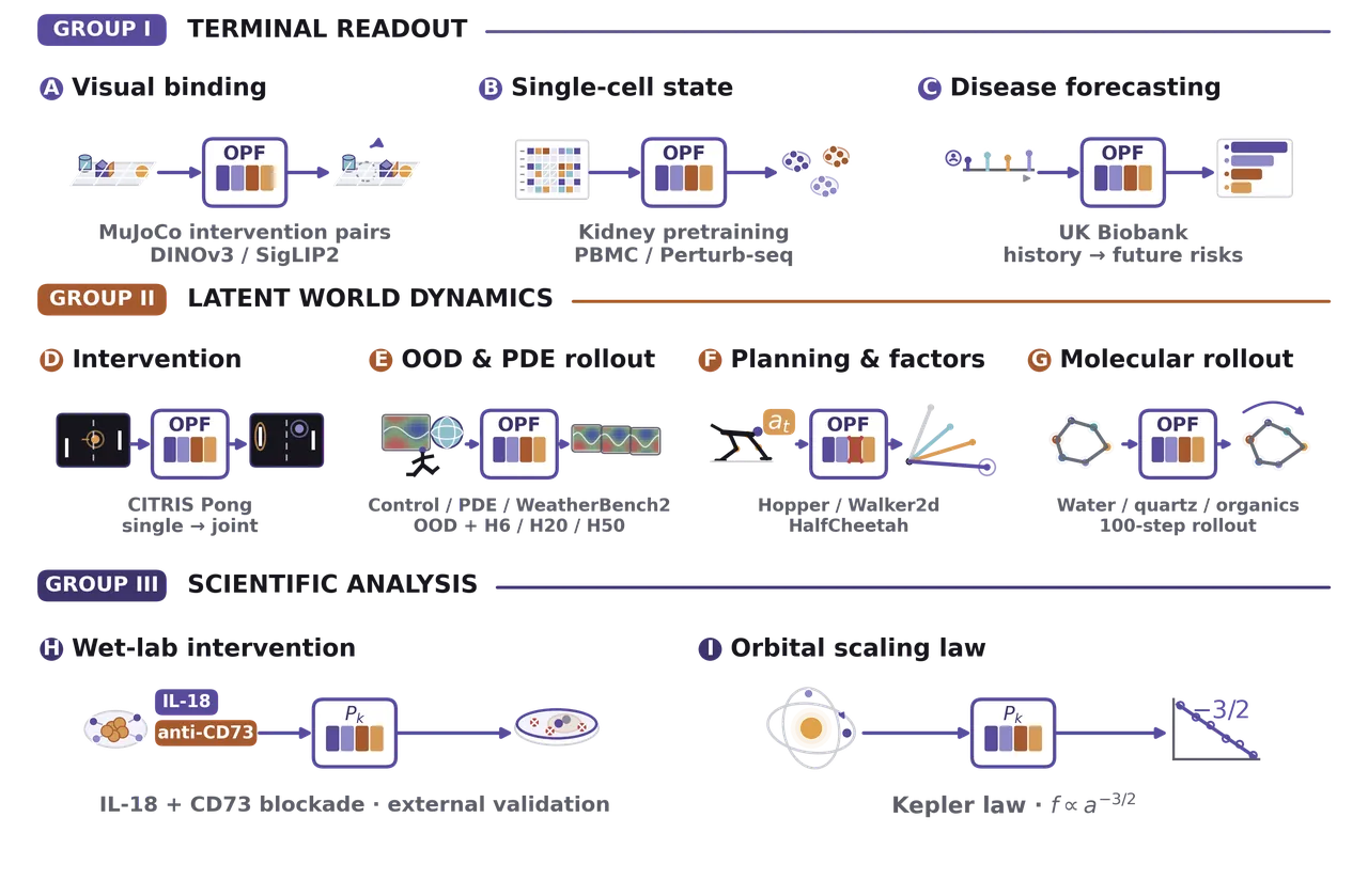
Figure 2: Scenario atlas. Each domain keeps its own context, target, encoder, and evaluation protocol while sharing the factorized predictive-state interface.

4. Three downstream uses of the same state

For ordinary readout tasks, the EMA encoder, projectors, and prediction heads are discarded. The online encoder is retained, and a domain-specific readout is attached:

$$h_{\delta,\tau}(x)=R_{\delta,\tau}\left(f_{\theta}^{\delta}(\mathcal{A}_{\delta}(x))\right).$$

The readout can pool a sequence, select a token, preserve a time index, or train a light probe. Here OPF shapes the encoder but the downstream task does not have to consume factors explicitly.

For future prediction, intervention modeling, planning, and simulation, the projectors and predictors remain active. The synthesized state is passed to a decoder, planner, or the next transition. For scientific analysis, the retained projections expose $u_k(x)=P_k^\top z_{\delta}(x)$ as a diagnostic interface. The paper uses that interface to nominate a biological intervention and to compare latent modes with a known orbital scaling law.

Paper-to-Code Correspondence

The public repository commit is c6e6c88f3ef75a4ce7acd660d6fa5779d995512c. Its core package deliberately exposes tensor-level operations rather than a one-click training pipeline. The state analysis and synthesis functions map directly to the equations above:

# jepa-anything-core/src/jepa_anything_core/opf.py:149
def decompose_state(state: Tensor, basis: Tensor) -> Tensor:
    ...
    return torch.einsum("...d,krd->...kr", state, basis)

# jepa-anything-core/src/jepa_anything_core/opf.py:167
def compose_state(factors: Tensor, basis: Tensor) -> Tensor:
    ...
    synthesis = torch.linalg.pinv(flat)
    return torch.einsum("...a,da->...d", factors.flatten(start_dim=-2), synthesis)

This code corresponds to Equations (3) and (5). The library also separates operational pseudoinverse synthesis from transpose synthesis used for geometry audits. Transpose synthesis is exact only when the basis is orthonormal, so its error becomes a useful diagnostic rather than a hidden implementation detail.

The second correspondence is the loss implementation. The library applies Gram constraints directly to the learned analysis rows and keeps statistical decorrelation as a separate diagnostic:

# jepa-anything-core/src/jepa_anything_core/losses.py:95
within_grams = torch.einsum("kad,kbd->kab", work, work)
within_penalties = (within_grams - identity).square().sum(dim=(-2, -1))

for first in range(num_factors):
    for second in range(first + 1, num_factors):
        cross_gram = work[first] @ work[second].transpose(0, 1)
        cross_penalties.append(cross_gram.square().sum())

This distinction matters. Geometric orthogonality, statistical decorrelation, and semantic independence are different properties. The repository states that factor coordinates remain anonymous unless separate experiments establish meaning. The paper follows the same boundary when it validates a biological factor through wet-lab work and an orbital mode through the Keplerian law.

The repository includes projection modules, loss functions, capacity-matched baselines, Welford variance tracking, and geometry audits with tests for QR initialization, pseudoinverse synthesis, low precision, reconstruction, and failure cases. Its README also states that the repository does not ship the paper's domain data, full training code, or trained weights. The implementation therefore verifies the method contract, not every empirical claim.

Experiments and Evidence

The paper evaluates the same core at three levels. Group I stops at a terminal readout: controlled visual binding, single-cell representation and perturbation prediction, and broad clinical event forecasting. Group II repeatedly feeds predicted states into intervention prediction, multi-step rollout, PDE simulation, and continuous-control planning. Group III retains factor coordinates for wet-lab validation and physical-law analysis.

Direct comparisons keep the adapter, encoder, context-target construction, optimization budget, data split, readout, and inherited base loss fixed. Standard JEPA uses one monolithic target, while JEPA-Anything adds OPF. The dimensions differ by domain, but the complete factorization constraint remains $Kr=d$.

Domain	State width $d$	Factors $K$	Factor width $r$	Main evaluation
Visual binding, MuJoCo	384 or 768	4	96 or 192	Injection, collapse, grid recovery
Single cell, Norman	512	4	128	AvgBIO, Pearson correlation
Clinical events	768	4	192	PRAUC over more than 1,000 events
CITRIS interventions	160	5	32	One-step and six-step four-channel MSE
Dynamics and PDEs	128	4	32	OOD, six-step, and long-rollout MSE
Continuous control	32	4	8	CEM return in the real environment
Molecular dynamics	64 channels	4	16	One-step MAE, 100-step RMSD

The visual experiments use DINOv3 ViT-S and SigLIP2 Base. Under the same learned-grid readout, JEPA-Anything improves injective accuracy and grid recovery while reducing collapse. For DINOv3, INJ rises from .572 to .581, Coll. falls from .426 to .417, and Rec. rises from .645 to .659. For SigLIP2, the corresponding values move from .483 to .490, .514 to .503, and .679 to .688.

The single-cell experiment pretrains on roughly 800,000 human kidney cells, evaluates PBMC-10K clustering in fine-tuned and zero-shot settings, and tests perturbation-response prediction on Adamson and Norman. The factorized model improves every reported metric:

Model	PBMC fine-tuned AvgBIO	PBMC zero-shot AvgBIO	Norman Pearson	Adamson Pearson
scGPT	0.7531	0.5288	0.631	0.905
Cell-JEPA	0.7830	0.7194	0.787	0.937
JEPA-Anything	0.8301	0.7752	0.814	0.942

The clinical model predicts a synthesized future patient state and ranks more than a thousand event risks by PRAUC on a fixed patient-level split. JEPA-Anything improves the mean ranking over matched monolithic JEPA. The result is important because the event distribution is broad and many outcomes are rare; aggregate accuracy would hide much of that behavior.

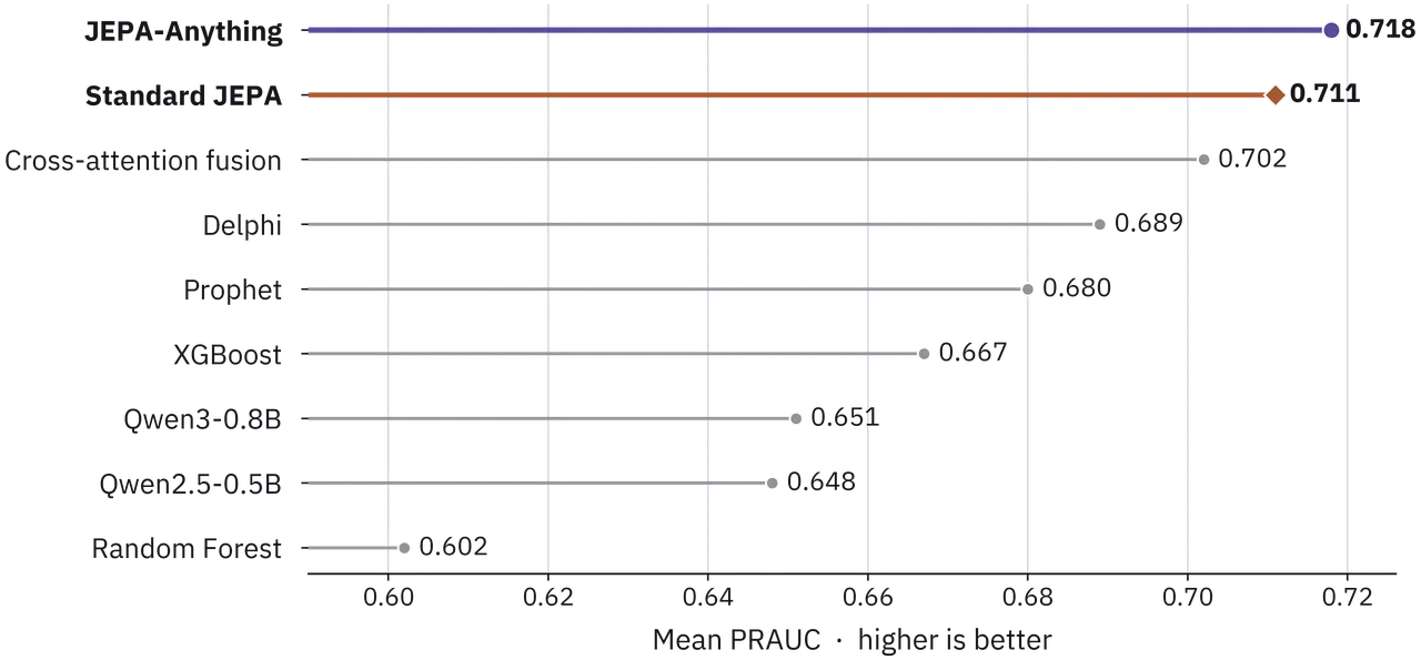
Figure 3: Broad-spectrum prediction of more than 1,000 future clinical events. Methods are ranked by mean PRAUC on the same cohort split.

CITRIS Interventional Pong tests both single interventions and withheld combinations. Relative to standard JEPA, one-step single-intervention MSE falls from 0.009541 to 0.006218, a 34.83% reduction. Combined-intervention MSE falls from 0.009441 to 0.008223, a 12.90% reduction, and six-step free-rollout MSE falls from 0.009478 to 0.008665, an 8.58% reduction. The compositional result suggests that the model reuses learned state-change rules instead of memorizing complete intervention patterns.

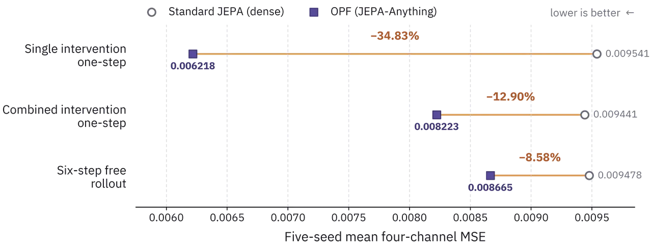
Figure 4: Intervention-conditioned prediction and free rollout on CITRIS Interventional Pong. Four-channel MSE is lower-is-better.

The mechanism audit makes the geometric effect visible. Unconstrained multi-head factors have a cross-factor subspace overlap of 0.4550, a minimum singular value of 0.00513, a condition number of 438.52, and transpose-synthesis NMSE of 0.7886. Orthogonal factorization reduces overlap to approximately $5.18\times10^{-16}$, raises the minimum singular value to 0.999989, reduces the condition number to about 1.00005, and lowers transpose-synthesis NMSE to approximately $2.98\times10^{-14}$. The factors therefore become a non-overlapping, unit-conditioned state coordinate system.

The ten-task dynamics benchmark covers CausalWorld, DeepMind Control, PDEBench, and WeatherBench2 with five seeds. All four representative systems have lower six-step errors. For PDEBench Burgers, step-one MSE falls from 0.001830 to 0.001101 and step-six MSE falls from 0.006369 to 0.004014. For shallow water, the corresponding errors fall from 0.007090 to 0.003999 and from 0.010510 to 0.006522.

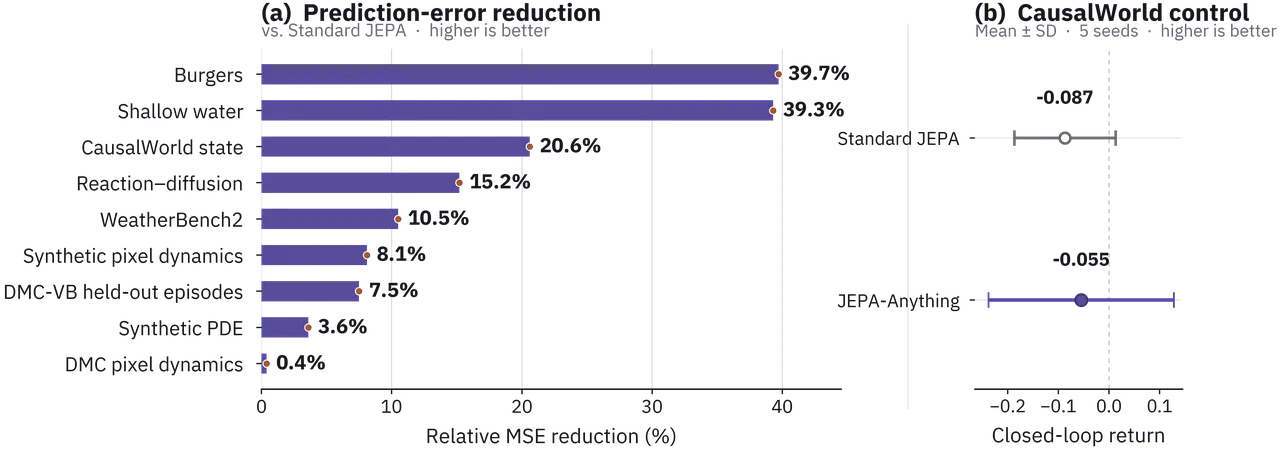
Figure 5: Ten-task matched dynamics benchmark. The left panel shows relative MSE changes; the right panel shows CausalWorld closed-loop return.

System and metric	Standard JEPA	JEPA-Anything	Change
Burgers held-out late MSE	0.16621	0.08389	About 49.5% lower
Burgers six-step MSE	0.29186	0.16153	About 44.7% lower
Kuramoto-Sivashinsky late MSE	1.1012	0.9558	About 13.2% lower
Molecular systems with best result	0/4	4/4	Best in all four systems

The long-rollout Burgers study extends the evaluation to 20 and 50 steps. JEPA-Anything reduces in-distribution error by 5.84% at H20 and 3.15% at H50. On high-frequency OOD trajectories, the reductions are 5.01% and 2.82%. The advantage persists but narrows at longer horizons, showing that better state geometry limits amplification without solving long-term dynamics errors.

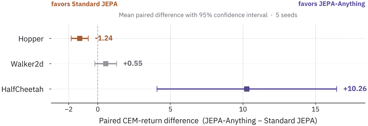
Figure 6: Capacity-matched continuous-control planning. Positive values favor JEPA-Anything; Hopper is the exception.

The control result is more conditional. JEPA-Anything improves mean CEM return on Walker2d and HalfCheetah, while Hopper favors standard JEPA. Factor activity remains healthy across all tested locomotion checkpoints: factor standard deviations are roughly 0.692-0.715 on Hopper, 0.587-0.601 on Walker2d, and 0.673-0.678 on HalfCheetah. Replacing a factor with its training mean increases rollout error, and for HalfCheetah, masking F1 or F3 lowers real-environment return in all five training seeds.

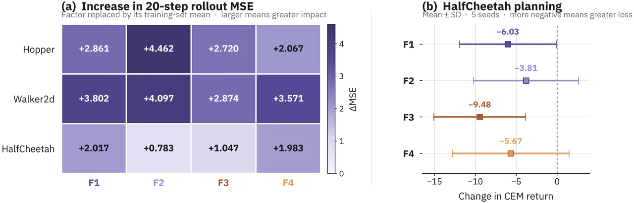
Figure 7: Factor-wise functional interventions. The panels report rollout-MSE increases and real-environment HalfCheetah return changes.

The molecular experiments use a TrajCast-style O(3)-equivariant model and apply OPF to the 64-channel multiplicity axis of the $l=1$ sector. JEPA-Anything obtains the lowest one-step MAE and 100-step final-position RMSD for water, quartz, paracetamol, and benzene. The 100-step RMSD values are 2.459, 1.877, 1.776, and 0.0645, respectively. In biology, factor analysis nominates IL-18 plus CD73 blockade, which receives support in Huh7-PBMC co-culture, patient-derived organoids, tumor fragments, and immunocompetent mice. In orbital data, spectral modes recover the Kepler relation $f\propto a^{-3/2}$ with fitted slope -1.4991 and $R^2=0.9999999$.

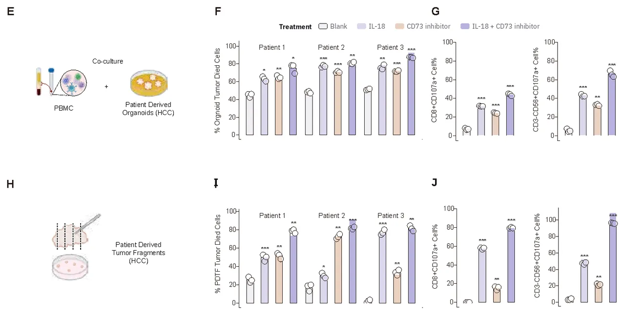
Figure 8: Selected wet-lab results in patient-derived hepatocellular carcinoma organoids and tumor fragments. The IL-18 plus CD73 blockade combination shows the strongest tumor-cell killing among tested conditions.

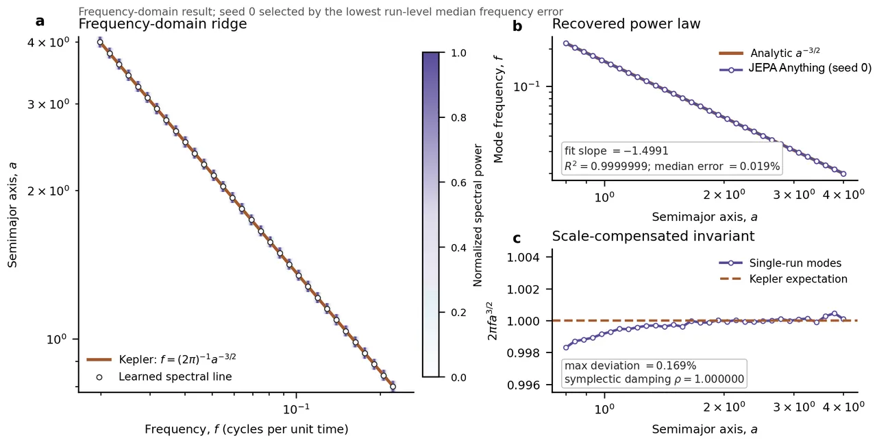
Figure 9: A physical-law diagnostic based on predictive latent modes. The learned spectral modes recover the Keplerian ridge with fitted slope -1.4991 and an $R^2$ close to one.

What the Work Changes

The strongest idea is not a universal encoder. It is the separation between domain-specific observation construction and a shared predictive-capacity layer. Different worlds keep different adapters, targets, and backbone architectures. What they share is the factorized state contract, the additive objective, and the rules for synthesis. The word "Anything" describes interface breadth, not identical weights or zero-shot transfer.

For robot learning, the work makes world-model structure testable. Orthogonality and condition number can reveal whether multiple prediction branches cover distinct state directions. Activity and masking tests can show whether a branch actually contributes to rollout or planning. This evidence chain is closer to operational model quality than a single next-step loss, especially in model predictive control where latent errors are reused repeatedly.

For scientific discovery, the paper treats learned factors as hypotheses rather than causal facts. The biological intervention and the Keplerian diagnostic show how factor coordinates can be checked against external evidence. The distinction is necessary because orthogonal, uncorrelated, and semantically independent are not equivalent.

Limitations and Risks

First, every domain still needs its own data, encoder, adapter, training budget, and base objective. The shared predictive core does not eliminate domain engineering or imply zero-shot transfer across worlds. A common interface is not the same as a common model.

Second, the public repository is narrower than the paper. It contains OPF primitives, baselines, loss functions, audits, and tests, but not the full experimental datasets, training pipelines, or trained model weights. A reader can verify the mathematical contract but cannot reproduce all reported tables from the repository alone.

Third, continuous-control gains are environment-dependent. Walker2d and HalfCheetah improve on average, while Hopper favors the baseline. Factor masking shows that all factors contribute to rollout, but not that four factors are optimal for every environment. $K$, $r$, and the regularization weights may need domain-specific calibration.

Fourth, long-horizon error still accumulates. The Burgers advantage shrinks from H20 to H50, and the high-frequency OOD gain narrows from 5.01% to 2.82%. Orthogonal synthesis controls how factor errors are amplified; it does not make the learned transition model accurate outside its training distribution or provide calibrated failure detection.

Fifth, orthogonal factors are not automatically semantic or causal. The paper uses external experiments to support selected interpretations, but a factor can encode multiple variables or change meaning across tasks. Naming a coordinate after a physical or biological concept requires separate evidence.

Conclusion

JEPA-Anything separates world modeling into a domain adaptation layer and a shared OPF predictive core. The core partitions target capacity into orthogonal factors, keeps those factors active, predicts them with dedicated pathways, and reconstructs a complete latent state. Terminal readout, recursive dynamics, planning, and scientific analysis then consume the same state interface in different ways.

The paper's contribution is broader than a single benchmark gain. It offers a testable design principle: factors should be non-overlapping, active, numerically stable to synthesize, and functionally useful under intervention. For embodied AI, that is a direct route toward world models that can be diagnosed rather than treated as opaque predictors. For cross-domain science, it connects predictive representations to external experiments and known physical laws.