PAPER DEEP DIVE
Generate, Track, Improve: Perceptive Multi-Skill Humanoid Locomotion with RL-Fine-Tuned Motion Generators
General purpose humanoids require locomotion controllers that are multi-skill, perceptive, dynamic, and robust enough to go anywhere humans can. In this work, we present a two layer locomotion architecture: (1) a perceptive flow matching motion generator plans whole body trajectories from raw depth images while a (2) perceptive tracking policy trained with control-guided RL follows these motions. Both policies are trained on a library of terrain consistent motion clips created with dynamically optimized human data which yields both accurate velocity tracking and terrain consistent references. Our central contribution is a simple yet effective off-policy RL fine tuning loop that improves the motion generator. A structured search method is used with the generator to gather data for advantage weighted regression. This off-policy loop is much more sample efficient than on-policy residual fine tuning and improves terrain consistency on unseen geometries and skill compositions. We find that successful terrain traversals increased by up to 25 percentage points and skill selection improved by up to 80 percentage points. By using raw depth images to perceive the environment no odometry or height maps are needed, and outdoor deployment is easy. With two cameras, the policy can see terrain coming from further away and adjust its velocity regardless of the commanded speed so it can traverse the terrain. A single policy pair enables a Unitree G1 humanoid to walk, run, stand, jump on and off of boxes, and traverse stairs in outdoor environments. Project page: https://zolkin1.github.io/generate-track-improve/
TL;DR
The system splits perceptive locomotion into two layers: a 26.8M-parameter flow-matching Transformer that turns two raw depth images plus a velocity command into a 1.24 s whole-body reference trajectory every 0.24 s, and a 50 Hz CLF-RL tracker that executes it. The contribution that matters is an offline RL loop that improves the generator itself. Closed-loop rollouts explore by perturbing the conditioning and the flow-matching initial noise instead of the 2,728-dimensional action, a critic fitted by value iteration labels advantages against true sampled returns, and advantage-weighted regression writes those improvements back into the generator's own weights. On out-of-distribution terrain and skill combinations this raises success by up to 25 points and lifts correct mode selection from 0% to about 80%, while a PPO residual baseline burns more than 160x the data and 30x the wall clock and still lands about 13 points behind.
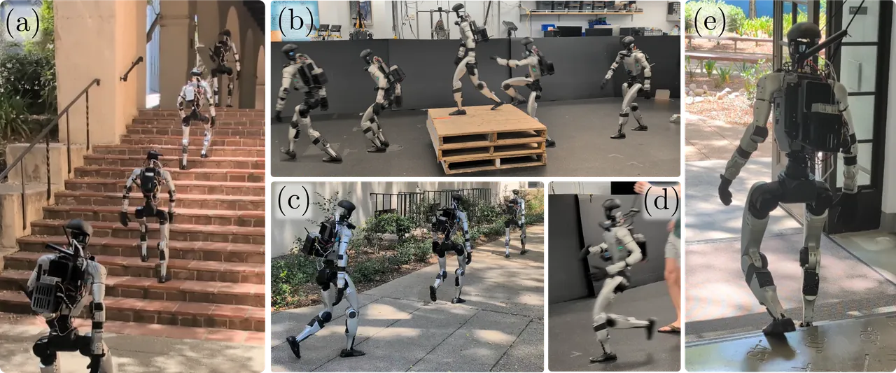
Figure 1: The perceptive control pair deployed on real terrain, indoors and outdoors. (a) Climbing 15 real stairs, including the transitions into and out of the staircase; (b) jumping onto a box, walking across, jumping down; (c) outdoor walking, including a turn onto a path; (d) indoor running; (e) descending real stairs.
Background: What Humanoids Lack Is Not a Skill but a Terrain-Aware Multi-Skill Controller
The paper opens with a blunt claim: the diversity of required skills combined with the perceptive dependence of real-world locomotion is why humanoids still do not show up doing reliable work in real scenes. Walking, running, parkour, and stair traversal have each been studied on their own, and capability in each has grown fast, but both research threads are missing a piece. Terrain-aware locomotion policies are typically not designed to scale to general whole-body control or to multi-velocity locomotion, so the robot struggles to go anywhere at a commanded speed in the real world and struggles further to extend into interaction skills such as opening a door or pressing an elevator button. On the other side, general whole-body controllers in the mimic family (SONIC and its relatives) track a great many motions but lack the perception and the terrain-aware motions needed to traverse the real world. This paper's stated job is to join the two: a pair of perceptive policies, one generating terrain-aware references and one tracking them in real time.
Why the generator-plus-tracker paradigm at all? The reasons the paper gives are engineering reasons, not performance reasons. Compared with distilling many experts, or having one generator emit both a kinematic trajectory and the actions to realize it, the layered architecture buys modularity and skill extensibility: as long as the tracking controller is general enough, adding a skill means adding reference clips to a motion library rather than retraining the tracker. It also supplies a natural compute split, with a lightweight tracker running at high frequency and a large motion generator queried at low frequency. That split is decisive at deployment: generator inference here takes about 11 ms while the tracker takes under 1 ms, an order of magnitude apart, which matches the 0.24 s planning period against the 0.02 s control period exactly.
The choice of perceptive input is a deployment trade-off of the same kind. Perceptive locomotion broadly has two routes: height fields, or raw sensor measurements. Height fields are awkward to deploy because they generally require a mapping package plus odometry. This paper takes the raw-depth route, which costs a simulated depth sensor and forces the network outputs to be observable within the camera's field of view. What it buys is no odometry and no height map, so moving outdoors is nearly free: the same policy pair runs indoors and outdoors in this paper with no terrain-specific tuning of any kind.
The authors are also careful to separate their work from prior generator-tracker systems. SONIC pairs a kinematic generator with a general tracking policy, but the generator is not perceptive and is flat-ground only. PARC proposes a perceptive generate-and-track pipeline that can produce new motions from a limited seed set, but it was never run on hardware, only on simulated characters, and it needs a kinematic correction step, a dynamic correction step, and diffusion policy training, so three iterations take about a month, clearly slower than the method here. Another closely related line requires odometry and a height scan, shows neither accurate velocity tracking nor outdoor experiments, and adapts by fine-tuning the tracker. This paper's position is: raw depth cameras, no odometry, demonstrated velocity accuracy, and a pipeline that improves the generator with RL, because some problems, such as which skill to use to clear an obstacle, cannot be fixed by fine-tuning the tracker at all.
The last piece of background is RL applied to flow-matching and diffusion policies. That has precedent in VLAs and in smaller behavior-cloned manipulation policies for legged and wheeled systems: one line uses the online algorithm DPPO over a reduced action space that does not command the legs directly, another freezes the generator and learns residual actions or steers latent noise. This paper's setting differs from both: the application is dynamic locomotion, and it adjusts the generator's own weights rather than bolting a residual on top. That distinction is exactly what motivates the PPO residual comparison later.
Preliminaries: The Mimic Route, CLF-RL, and Flow Matching
The dominant recipe for humanoid whole-body control is mimic: start from a reference trajectory, then use RL to learn a controller that tracks it. The route is attractive because performance is good, results look clean, and reward shaping is nearly unnecessary. The cost is that a reference trajectory has to exist first. Sources include human motion capture, reduced-order models, dynamically optimized trajectories, and animation data. Many mimic controllers stop at motion playback, however, and lack general skills plus an interface that a higher autonomy stack can actually call. In locomotion that interface is usually velocity conditioning, periodic orbit construction, or a reduced-order model that can be queried in real time so the robot follows a commanded velocity, which is precisely what an upstream navigation policy emits. The data pipeline in this paper has to satisfy two constraints at once: reference motions must be dynamically feasible and velocity-accurate, since data quality caps tracking accuracy, and they must be consistent with terrain, or feet clip through geometry or miss it entirely.
The tracking layer uses a variant of CLF-RL. CLF-RL encodes convergence of tracking error into the reward structure through a control Lyapunov function, and the authors picked it because prior work reports lower tracking error. Their variant changes two things: the tracking targets are the body positions of every link rather than joint angles, and a scaling term $S$ is introduced to fix numerical conditioning without giving up the CLF property. Proposition 1 in the appendix proves that this is legitimate. With $A_\eta,B_\eta$ block-diagonal by output, $Q,R$ diagonal positive definite, and $P$ the stabilizing solution of the corresponding CARE, then for any $S=\mathrm{diag}(a_1,b_1,\dots,a_n,b_n)$ with $a_i,b_i>0$,
$$\bar{V}(\eta)=\eta^{\top}SPS\eta$$
is still an exponentially stabilizing CLF. The proof turns on the CARE decoupling by output, so that $S_iA_iS_i^{-1}=c_iA_i$ with $c_i=a_i/b_i$ absorbs the scaling into equivalent weights $\bar{Q}_i=c_iS_iQ_iS_i$ and $\bar{r}_i=\tfrac{b_i^3}{a_i}r_i>0$. In plain terms, the authors gain free rein over per-channel weighting without breaking the stability guarantee, which is why CLF's inherent bias toward velocity terms can be suppressed here: velocity has larger variance than position, so weighting it aggressively is not the right default.
The generation layer uses flow matching. During training, noise $x_0\sim\mathcal{N}(0,I)$ and data $x_1$ are linearly interpolated into $x_t=(1-t)x_0+tx_1$, and the network learns a velocity field that fits the constant field $v^{*}=x_1-x_0$; inference integrates numerically from noise, here with 8 Euler steps. Flow matching is chosen over autoregressive token generation so that a full whole-body trajectory can be emitted in one shot inside a 0.24 s planning period. The fact that the initial noise $x_0$ is a sampleable continuous quantity later becomes the handle for structured search in RL fine-tuning.
Method
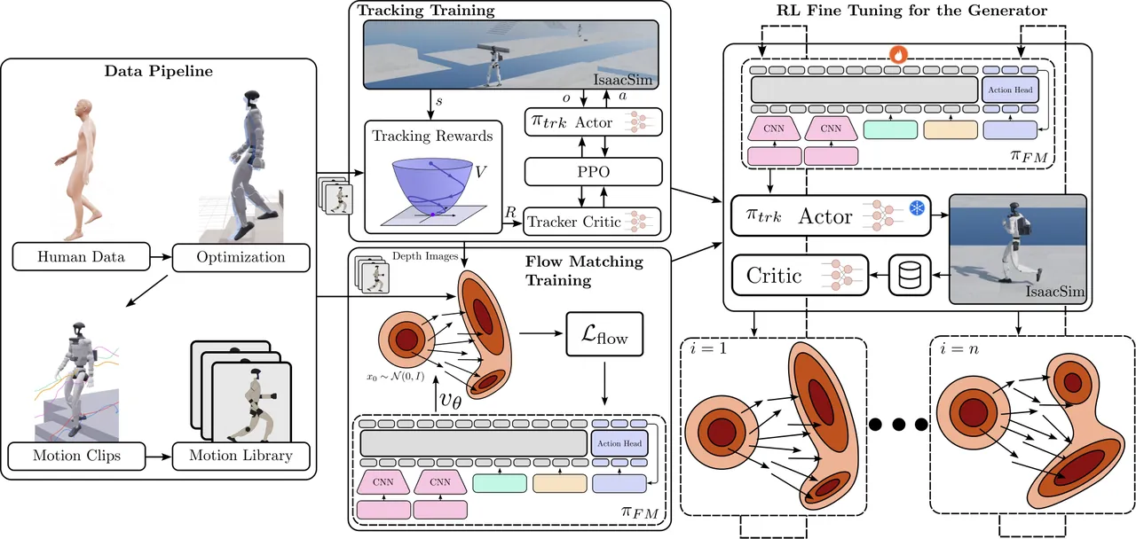
Figure 2: Method overview. Human motion data is optimized and passed through a generative model to build a library of motion clips; a perceptive tracking policy is trained with CLF-RL; that library plus the tracker are then used to collect the depth images the robot will really see, which together with velocity commands and the library form the supervised training data for the flow-matching generator (flow MSE loss); finally the generator is fine-tuned with offline RL, where generator and tracker roll out in closed loop into a buffer, a critic estimates infinite-horizon return, advantages label the data, and advantage-weighted regression shifts the generator's output distribution. The resulting policy pair is deployed on hardware for perceptive locomotion.
1. System Overview: 50 Hz Tracking, Re-planning Every 0.24 s
The method has four stages: data pipeline, tracker training, generator training, and RL fine-tuning of the generator. What gets deployed is two separate policies. The tracker runs at 50 Hz, the usual rate for an RL control policy, while the generator is queried every 0.24 s, that is, every 12 control steps. The input split is clean: the tracker consumes proprioception plus one depth image and outputs joint position targets; the generator consumes the desired velocity, its own previous output, and two depth images, and outputs a 1.24 s whole-body trajectory. The data pipeline supplies terrain-consistent reference motions for both, and fine-tuning improves the generator only after it has already been trained.
The frequency gap carries a benefit that is easy to miss. The generator emits a trajectory covering the next 1.24 s but only refreshes every 0.24 s, so consecutive plans overlap roughly five-fold. The tracker always has a complete reference to follow through that overlap, which means generator inference latency (11 ms) and camera-pipeline latency do not turn directly into a control hole. The paper still stresses that shortening the sensor-input-to-new-trajectory delay remains critical for dynamic motions.
2. The Motion Clip Pipeline: Dynamic Optimization Plus Motion Bricks In-Betweening
The tracking policy needs pre-built terrain-aware motion clips. The seed is human motion capture from the bones-seed dataset, which the authors turn into optimized humanoid reference motions: 252 flat-ground steady-state references (forward and backward straight walking, diagonal walking, turning walks, in-place turning, lateral stepping, straight running, turning runs) covering omnidirectional capability, plus 46 references for jumping onto and off boxes and for ascending and descending stairs.
The optimization is a multiple-shooting, state-constrained formulation with MuJoCo as the dynamics backend. The rationale is specific: because MuJoCo's contact dynamics can be differentiated through, the contact schedule is allowed to shift slightly, while multiple shooting supplies numerical stability on its own. State constraints are the key capability here, since they let the authors impose periodicity (final state equals initial state) and average velocity (the reference is dialed to the target speed exactly).
Terrain motions have no terrain ground truth in the open bones-seed data, so the authors invert the problem and place the terrain first: terrain is arranged to match the motion, and the same optimization is solved in a MuJoCo scene containing it. After that first solve, contact ground truth falls out of the simulation, obtained by thresholding contact forces on the relevant end-effector bodies and filtering out overly short contact and non-contact segments. The authors point out that this is more reliable than detecting contact kinematically, and it is a direct side benefit of doing dynamic optimization. With contact ground truth in hand, the robot can be kinematically retargeted across many terrain dimensions, which matters because a dataset can never cover every dimension found in the real world: foot offsets are computed so that feet land on the terrain at contact, those offsets are smoothly interpolated between adjacent contacts to produce a continuous end-effector trajectory deformation, and inverse kinematics recovers joint angles. After retargeting to a new height, the dynamic optimization is run again, yielding motions that are both feasible and smooth on terrain.
With that batch of optimized motions, full training clips can be generated. Clips run 6 to 20 s and are grouped by family: jump down, jump up, stairs down only, stairs up only, stairs down transition, stairs up transition, and flat ground. Generation samples a velocity profile, picks the steady-state optimized reference closest to each steady-state command, and then in-betweens with the generative model Motion Bricks. The authors note this step does what motion matching would also do, but faster and more smoothly. The output is 10,000 motion clips covering 140 distinct terrain tile geometries, synthesized into one motion library, so training sees many velocity profiles on the same geometry and many geometries at once.
3. The Tracking Policy: a CLF-RL Variant with a Self-Scanning Depth Input
The tracker's reward is two CLF-RL tracking terms plus penalties for undesired contact, torque limits, joint limits, action rate, and torque magnitude. It is a perceptive policy, and its input includes a depth scan that sees the robot's own body: only 30x26 pixels, downsampled on hardware from a 600p image. Table 1 gives the full observation layout.
| Observation | Dim | History stack |
|---|---|---|
| Joint angles | 29 | 10x |
| Joint velocities | 29 | 10x |
| Projected gravity | 3 | 10x |
| Root angular velocity | 3 | 10x |
| Previous action | 29 | 10x |
| Lower depth camera | 780 | none |
| Reference trajectory | 572 | none |
| Velocity command | 39 | none |
Table 1 (paper Table I): tracker observation terms and dimensions. History terms are stacked over the indicated number of steps; 780 is the 30x26 depth scan.
The network is a two-stage feed-forward MLP: one MLP encodes the reference trajectory and the velocity command, and its output joins proprioception and the depth input in a second MLP, with ELU activations throughout. The reference/command MLP has hidden widths [1024, 512, 512]; the main MLP is [1024, 512, 256, 128]. The policy outputs joint position targets at 50 Hz into joint-level PD controllers, with action rate and gains taken from prior work. For sim-to-real, physical quantities are domain randomized (center of mass, joint friction, ground restitution, camera angle and extrinsic offsets), and noise is added to the reference trajectory, the depth readings, and the proprioceptive inputs. Training runs in IsaacLab with 8,192 environments on one H100 for 20,000 iterations, about 48 hours, using PPO with an asymmetric actor-critic (RSL-RL implementation).
4. The Generator: a Flow-Matching Transformer with a Cacheable Prefix
The generator is an autoregressive-style flow-matching Transformer whose only sensor observation is depth. Depth images pass through a CNN into tokens that enter the Transformer, which also receives the velocity command and a trajectory history (a subset of nodes from the previously generated trajectory, one token per node); a flow-matching head outputs the reference trajectory. In terms of scale: each camera's CNN emits 56 tokens, so 112 perceptive tokens in total; the velocity command is spread over 13 tokens; the model has 8 layers of 8 heads, FFN width 2048, $d_{\text{model}}=512$, and 26.8M learnable parameters.
One decision in the attention structure is made specifically for the RL fine-tuning that comes later: the prefix tokens (depth, velocity command, history) fully self-attend, but the prefix does not attend to the output trajectory tokens in the flow-matching head, while the output tokens do attend to the prefix. This means the internal representations of depth, command, and history are independent of the current flow-matching velocity field, which buys two things: (1) the Transformer encoder can be reused directly by RL fine-tuning, with the critic freezing it and training only a value head; and (2) inference is faster, because the prefix encoder runs once and is then cached across all 8 integration steps. Perceptive tokens are positionally embedded by their angle within the camera's field of view.
The depth input to the CNN has five channels: the depth value, the pixel's $x$, $y$, and $z$ coordinates in 3D space, and a validity bit. Those coordinates live in a frame attached to the robot's root link that is gravity-aligned and yaw-aligned: it rotates with the robot's yaw but not with pitch or roll. They are computed by forward kinematics from root link to camera, then transforming depth pixel positions into the root frame, which is also the frame in which the flow-matching head outputs root node positions. The authors emphasize that because the generator receives no proprioception at all, these extra coordinate channels are what make it work on terrain. Without them the robot cannot distinguish certain situations, for example that it is falling toward the terrain, or that the terrain is approaching while the robot itself is not moving.
How the training data is collected is deliberate: the trained tracking policy follows the very motion clips it was trained on, and the depth images, the reference trajectory before that instant (as history) and after it (as the prediction target) are all recorded. Real RL rollouts are used rather than kinematic playback so that the states the depth camera visits are as realistic as possible. A buffer of past depth measurements is also maintained, and training deliberately draws an older frame instead of the newest one so the generator learns to tolerate camera latency. The dataset starts at 200k points and then undergoes one augmentation aimed at "the reference must be consistent with the terrain": every data point whose trajectory lies partly or wholly on terrain gets a random distance along the terrain plus a yaw offset applied to the robot state, the depth image is re-cast from the new position while the reference trajectory stays fixed, and 3 augmented copies are made per relevant point. In effect the data insists that these axes remain correct relative to terrain even as the robot moves.
Two further training details both serve autoregressive robustness. On 20% of points the history is replaced by a learnable null embedding, which both forces the policy to stop merely continuing whatever the history was doing and to genuinely learn the mapping from velocity command and depth to output trajectory, and supplies exactly the parameter needed for the first inference online, when no history exists yet. History trajectories are also noised during training so the policy is robust to its own outputs when it runs autoregressively. The observed result is that the final policy is very stable in autoregressive rollout despite never being trained on its own outputs, since the whole of training is teacher forcing. The generator trains for 100 epochs, about 12 hours on a single H100, and deploys with 8 Euler integration steps.
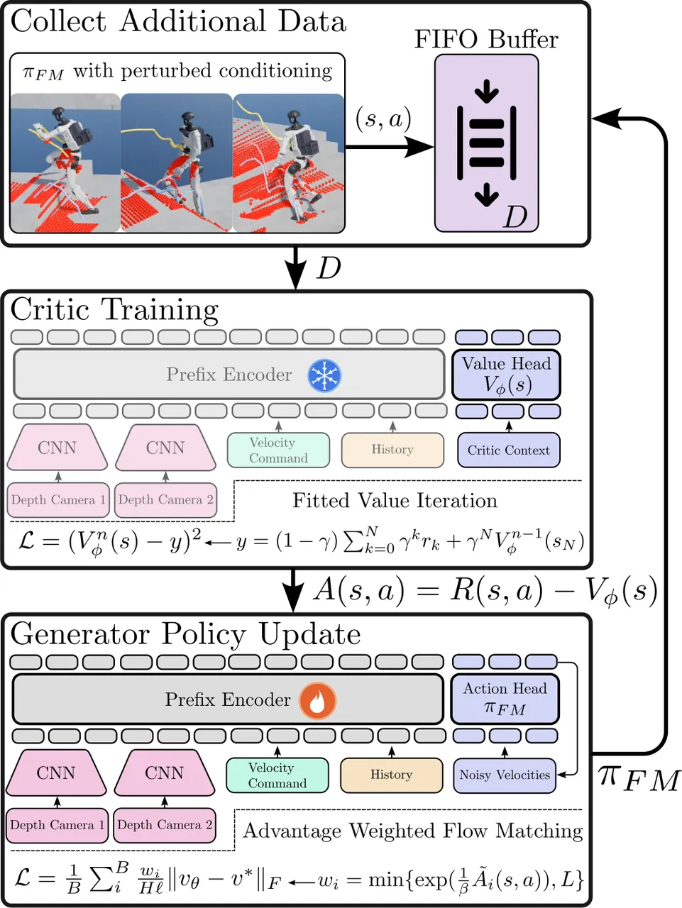
Figure 3: The RL fine-tuning architecture for the generator and the Transformer structure of the two networks. The overall flow is collect data, train the critic, update the generator; the right side marks that the prefix encoder is frozen during critic training and updated during the generator update, with the critic using a value head and the generator using the velocity-field action head.
5. Offline RL for the Generator: Treating the Tracker as Part of the Robot's Dynamics
After initial training the flow-matching policy already closes the loop with the tracker, but it still struggles on out-of-distribution combinations of terrain and task. The authors choose to fine-tune the generator rather than the tracker. Formalized as an MDP with states $s_k\in\mathcal{S}$ and actions $a_k\in\mathcal{A}$, the index $k$ counts re-planning steps, and because the tracking policy is frozen, "from the perspective of this MDP, the tracker is effectively part of the dynamics of the robot rather than something to be tuned." The state is the full conditioning (depth scan, reference history, velocity command) and the action is the entire trajectory, so $\mathcal{A}\subset\mathbb{R}^{H\times\ell}$ with $H=62$ nodes of $\ell=44$ dimensions each, $H\times\ell=2728$. The policy gives sampled actions $a_k\sim\pi_{FM}(a|s_k)$, per-step rewards are $r_k=r(s_k,a_k)$, trajectories are $\tau=\{(s_0,a_0),(s_1,a_1),\dots\}$, and the infinite-horizon discounted return is
$$J_{\pi_{FM}}(s)=\sum_{k=0}^{\infty}\gamma^{k}r_{k}$$
Why not just run PPO? The reason given is search efficiency: at every re-plan the generator emits close to 3,000 numbers, a full whole-body trajectory, and adding independent Gaussian noise to those outputs does not produce anything resembling a structurally valid trajectory, so the search is nearly useless. The alternative here is structured search: do not perturb the action, and instead (1) perturb the conditioning during rollout so the robot is shown other, still-plausible actions, (2) spawn the robot into positions the original policy would never have reached, and (3) perturb the initial sampling noise of the flow-matching process. This jumps between modes without ever adding noise to the action. When conditioning is perturbed, the nominal, unperturbed conditioning is still stored, so policy training treats the nominal action as a valid action in the state the robot actually occupied.
Rewards are laid out in Table 2 and follow one principle: terrain consistency first, velocity tracking and success second. The penetration term penalizes body points intersecting terrain; the contact term penalizes bodies that a kinematic classifier says should be in contact but are too deep or too far away; velocity tracking and success are both modulated by terrain consistency and only pay out meaningfully when consistency is good. Since deviating from the commanded velocity is often necessary when clearing an obstacle, this modulation lets both be rewarded consistently. The success reward is additionally gated by the worst terrain consistency over the whole episode, so a strong signal appears only when every plan in the episode was terrain-consistent.
| Reward term | Expression | Purpose |
|---|---|---|
| Terrain penetration $r_{pen}$ | $\sum_{b=1}^{N_b}w_b\sum_{p\in P(b)}-\min\{\text{sdf}(p),0\}$ | Penalizes body points that enter the terrain |
| Terrain contact $r_{con}$ | $\sum_{b=1}^{N_b}c_b\min_{p\in P(b)}|\text{sdf}(p)|$ | Penalizes bodies that should be in contact but are too far or too deep |
| Terrain consistency $r_{terr}$ | $\exp(-(w_c r_{con}+w_p r_{pen}))$ | Squashes both terms into (0,1] and serves as the primary reward |
| Velocity tracking $r_{vel}$ | $\sin(\frac{\pi}{2}(r_{terr})^{s_{vel}})\exp(-|v_x-v_x^{cmd}|/\sigma)$ | Velocity accuracy modulated by terrain consistency |
| Success $r_{succ}$ | $\sin(\frac{\pi}{2}(\min_k r_{terr})^{s_{succ}})\cdot C1_{reached}$ | Arrival reward gated by the worst consistency in the episode |
| Total | $r_{terr}+r_{vel}+r_{succ}$ | - |
Table 2 (paper Table II): rewards for generator RL. $N_b$ is the number of body links, $P(b)$ is the point set on a body, $\text{sdf}(p)$ is the terrain signed-distance value at that point, and $s_{vel}$, $s_{succ}$ tune how sharply the terrain term decays. These rewards are inspired by PARC.
Data collection happens in IsaacLab with the flow-matching policy driving a fixed tracking policy in closed loop. The authors note an important side effect: from this point on the pre-made motion clips can be discarded and fine-tuning can proceed on any terrain. The buffer is a FIFO of capacity $D$: 2,000 episodes of data points (re-plans) are collected initially, and each later iteration adds 500 more episodes while ejecting the oldest 500.
The method depends on advantage estimates to decide which state-action pairs are better, so a critic must be fitted to predict the infinite-horizon discounted return $J_{\pi_{FM}}(s)$. It is trained by fitted value iteration and reuses the generator's own frozen prefix encoder, training only a value head. FVI iteration 0 uses a non-bootstrapped Monte-Carlo estimate $V(s_i)\approx\sum_{k=i}^{\infty}r_k$, with termination truncating the rollout: if step $k$ terminates in failure, all subsequent rewards are recorded as zero; if the robot has not fallen, the rollout is still truncated but bootstrapped with a tail value equal to the reward at the last step. Iterations $n>0$ look ahead $N$ steps and bootstrap with the previous $V$, regressing onto values scaled by $(1-\gamma)$ so that the target has the same units as the reward:
$$V^{n}(s)=(1-\gamma)\sum_{k=0}^{N-1}\gamma^{k}r_{k}+\gamma^{N}V^{n-1}(s_{N})$$
Once FVI finishes, the critic labels advantages as $A(s,a)=R(s,a)-V(s)$, where $R(s,a)$ is the true sampled return from that state: the trajectory is rolled out to termination with no bootstrapping and no use of the critic, so the advantage label always involves a real return. In practice the normalized advantage $\tilde{A}=A/\sigma_A$ is used, with $\sigma_A$ computed once per RL iteration so that the weighting coefficient $\beta$ downstream can be set in normalized units. There is also a leakage guard: two critics are trained, each on half the data, and each is used to label the advantages of the other half, because multiple data points inside one episode share the same success-or-failure label and a single critic could memorize episodes.
With advantages in hand, every data point gets a weight $w=\min\{\exp(\tfrac{1}{\beta}\tilde{A}(s,a)),\,L\}$ where $L$ caps it. Those weights go straight into the flow-matching MSE loss: sample $t\in[0,1]$ uniformly, sample initial noise $x_0\sim\mathcal{N}(0,I)$, interpolate to $x_t=(1-t)x_0+tx_1$, take the linear velocity field $v^{*}=x_1-x_0$, and the weighted loss is
$$\mathcal{L}=\frac{1}{B}\sum_{i}^{B}\frac{w_i}{H\ell}\left\|v_{\theta}(x_t^{i},t_i,s_i)-v^{*}\right\|_{F}^{2}$$
where $B$ is the batch size, $\|\cdot\|_F$ is the Frobenius norm, and dividing by $H\ell$ makes the loss independent of trajectory size. At this point the shape of the whole method is visible: exploration happens in the conditioning and the initial noise, while learning happens through supervised regression, so it avoids both an ineffective Gaussian search over a 2,728-dimensional action space and the sample waste of online algorithms.
New data drops into this loop easily. Pre-training data can participate in fine-tuning too, added to the flow-matching update with weight 1 but excluded from critic training and advantage labeling. That provides a knob against forgetting existing motions, and the multi-terrain fine-tuned policy later deployed on hardware was trained exactly this way. The full RL fine-tuning runs 5 iterations of 5 epochs each in the flow-matching update, about 6 hours on one H100, varying with terrain and episode length.
flowchart TD
  MOCAP["Human mocap, bones-seed"] --> OPT["MuJoCo multiple shooting + state constraints<br/>periodicity + average-velocity constraints<br/>252 flat + 46 terrain references"]
  OPT --> RETGT["Contact ground truth, then kinematic retargeting<br/>foot offsets + IK, dynamic optimization again"]
  RETGT --> MB["Motion Bricks in-betweening<br/>10,000 clips / 140 tile geometries"]
  MB --> TRK["Tracker: CLF-RL variant + depth scan<br/>IsaacLab 8192 envs / 20,000 iters / about 48h<br/>50 Hz joint position targets"]
  MB --> GEN["Generator: flow-matching Transformer, 26.8M<br/>100 epochs / about 12h<br/>200k points + 3 terrain augmentations each"]
  TRK --> ROLL["Closed-loop rollout, generator drives frozen tracker<br/>structured search: perturbed conditioning + spawn pose + initial noise"]
  GEN --> ROLL
  ROLL --> BUF["FIFO buffer<br/>2,000 episodes first, then +500 / eject 500 per iteration"]
  BUF --> CRITIC["Critic: frozen prefix encoder + value head, FVI<br/>two critics cross-label the other half of the data<br/>A(s,a) = R(s,a) - V(s)"]
  CRITIC --> AWR["AWR updates the generator weights<br/>w = min(exp(A_tilde / beta), L)"]
  AWR --> GEN
  AWR --> DEP["Deploy on Unitree G1 + Jetson Thor<br/>generator 11 ms / every 0.24 s<br/>tracker 50 Hz, under 1 ms"]
6. Deployment: Jetson Thor and the Division of Labor Between Two Depth Cameras
Both policies run on the onboard NVIDIA Jetson Thor: flow-matching inference is about 11 ms and the tracker is under 1 ms. Even though the generator is only queried every 0.24 s, the authors still stress that compressing the delay from sensor input to new trajectory matters for dynamic motions. The two cameras are a Zed X mini and a Zed X, both connected first to an NVIDIA Jetson Orin for depth processing and downsampling, then forwarded to the Thor over ROS2. Only the downsampled pixels are simulated during training, rather than simulating a full camera and downsampling inside the simulator, which cuts the cost of perceptive simulation substantially. For mounting, the Zed X sits high on the torso facing roughly forward, and the Zed X mini sits low on the torso where it sees the legs and the ground directly beneath the robot. Thor and Orin are both powered by the robot itself, and velocity commands arrive over a Bluetooth joystick.
Experiments
RL Fine-Tuning: up to +25 Points of Success Out of Distribution, Mode Selection from 0% to About 80%
To measure what fine-tuning contributes, the authors build four configurations: (1) boxes, one or two boxes of varying width and height; (2) stairs, ascending then descending, of varying width, with one or two walls on the sides, start and end platforms, and an intermediate landing between the up and down flights; (3) multi-terrain, mixing boxes, stairs, some in-distribution terrain, and a realistic building entry way (two flights of different dimensions, walls, and a landing between them); and (4) the in-distribution terrain set, that is, the terrain the generator and tracker were originally trained on. The first three are out of distribution for reasons including that the policy was never trained to both jump onto and jump off a box within one episode, that box widths were changed, that walls were added around stairs, and that the entry way is entirely new terrain. Success means reaching a goal region within the allotted time without falling, with goal regions distributed across the terrain.

Figure 4: The effect of RL fine-tuning on out-of-distribution and in-distribution terrain. (a) Success rate, improved by up to 25 points; (b) mean contact penalty, lower is better, indicating that fine-tuned policies are more terrain-consistent; (c) the fraction of whole episodes in which every mode (skill) was chosen correctly, for instance where a two-box terrain requires two jumps up and two jumps down. Fine-tuning helps most on mode selection: one stairs terrain goes from 0% correct to about 80%. Error bars are 95% confidence intervals.
The three panels give three independent pieces of evidence: success improves across the board, by up to 25 points; mean contact penalty falls, meaning trajectories fit the terrain better; and mode selection improves markedly. Mode here means the skill used to clear terrain, for example a stair trajectory versus a box-jump trajectory. The mode labeling protocol is worth recording separately: each policy is rolled out 50 times per terrain, all rollouts are shuffled to avoid bias, and a human labels the chosen mode one by one; if a human cannot tell which mode was used, it counts as incorrect. From this the authors draw a pointed conclusion: adjusting mode selection is something fine-tuning the tracker cannot do, so generator RL and tracker fine-tuning are complementary tools rather than alternatives.
What actually goes onto hardware is the multi-terrain fine-tuned version, which also validates that fine-tuning transfers across terrain types and across skills. That version was trained with pre-training data mixed in as described above, so the generator learns the new environment without forgetting its other motions.
Algorithm Comparison: AWR Matches or Beats Everything, While a PPO Residual Costs 160x the Data and Still Trails by 13 Points
The second experiment examines the choice of algorithm. This paper's method (AWR, advantage-weighted supervised regression over offline rollouts) is compared against four alternatives: filtered BC (filtered behavior cloning), arrival filtering (keep the data from every rollout that reached the goal region), plain BC / self-distillation, and AWR without perturbed conditioning. Plain BC removes all advantage information and asks whether merely having data on the new terrain helps, even without a critic or any filtering; the two filtering variants probe the filtering mechanism itself; and dropping conditioning perturbation isolates the contribution of that search strategy. The box terrain is further split into a strict termination variant (terminate when deviation from the generated trajectory exceeds 12 cm) and a loose one (30 cm threshold).
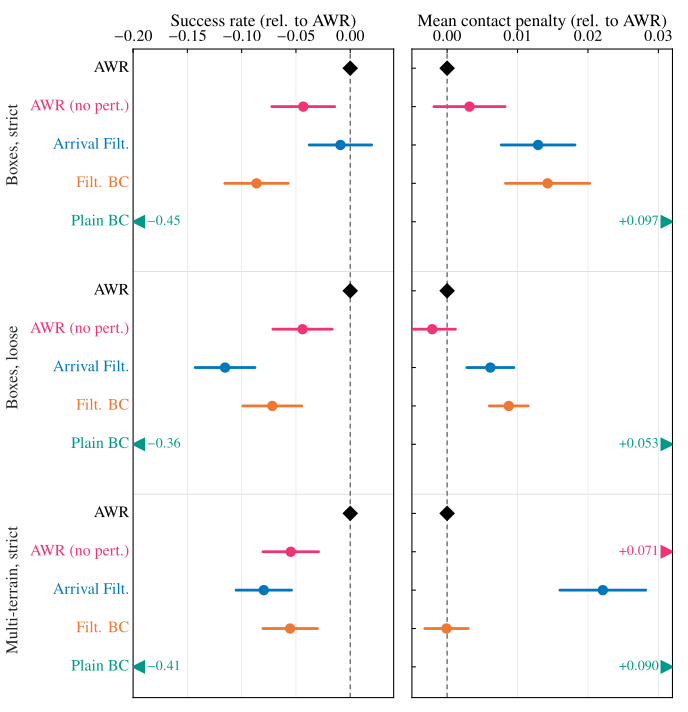
Figure 5: How alternative fine-tuning algorithms and search strategies compare with this paper's AWR, across terrains and across strict/loose termination on box terrain. AWR is equal or better on both success rate and terrain consistency. Error bars are 95% confidence intervals.
The result is that AWR consistently ties or wins on both success rate and terrain consistency, and each control says something distinct. Plain BC fails badly, so some advantage or filtering mechanism is necessary: having data on the new terrain is not enough on its own. Both filtering variants are worse overall. Arrival filtering is far more sensitive to the termination criterion, losing about 10 points of its success advantage relative to AWR when moving from strict to loose termination, while filtered BC trails AWR by a stable 5 to 10 points. The authors explain why arrival filtering does not collapse the way plain BC does: its termination criterion is based on tracking performance, so it implicitly improves the terrain consistency metric. Removing conditioning perturbation costs 4 to 6 points of success, produces clearly higher contact penalty on multi-terrain, and performs persistently worse on stairs terrain, which quantifies the contribution of structured search directly.
The comparison with an online algorithm is harder-edged. The authors train a residual policy with PPO: its observation is the generator's output plus the generator's own observation, it outputs a residual correction to the trajectory, its action space is the same dimension as the generator's full output, and its rewards are identical to the offline method's. If the residual approach worked, it could in principle be distilled back into the generator afterwards. The conclusion is that PPO is markedly less data efficient: training was stopped by the authors at 2,000 iterations, by which point it had consumed more than 160x the data and more than 30x the wall-clock time of the offline method, and its success rate was still about 13 points below AWR. The authors concede it may still have been on an upward trend, but climbing further would require far more data and compute, so the conclusion for this setting is that the offline algorithm (AWR) is the better RL fine-tuning route.
Velocity Tracking and Terrain Traversal: the Robot Decides When to Slow Down
One thing has to be stated up front: terrain cannot be traversed at arbitrary speed. There are no sprinting-up-stairs trajectories in the data and no ability to jump onto a box at high speed, so the robot slowing itself down is expected and necessary. What would be unacceptable is requiring the upstream command to supply the correct speed in order to clear an obstacle. The policy therefore has to modulate speed autonomously from depth: decelerate to a traversable speed when approaching terrain, then return to the commanded speed afterwards.
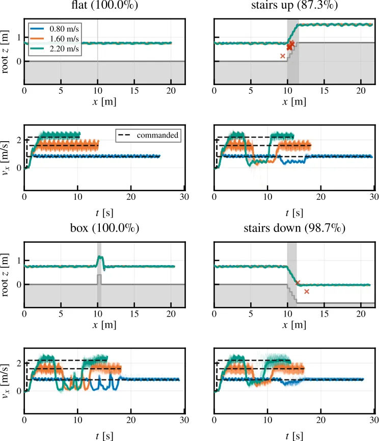
Figure 6: Traversal capability of the fine-tuned policy across many terrains, and how terrain affects robot speed. The robot decelerates autonomously on approach so it can traverse robustly, while overall velocity tracking stays accurate and traversal stays reliable. The percentages in the figure are success fractions over 150 samples per terrain.
Figure 6 answers two questions at once: whether the fine-tuned policy still holds its velocity tracking accuracy (conditioning perturbation was added during training, which could in principle have damaged it), and whether sim-to-sim holds, since evaluation is done in MuJoCo while training was done in IsaacLab, with 50 rollouts per speed and a different flow-matching sampling seed each time.
| Velocity command $v_x$ (m/s) | This pipeline, RMSE [95% CI] | Motion Bricks alone [95% CI] |
|---|---|---|
| (-1.0, -0.2] | 0.484 [0.357, 0.598] | 0.462 [0.346, 0.562] |
| (-0.2, +1.0] | 0.230 [0.191, 0.271] | 0.368 [0.308, 0.434] |
| (+1.0, +2.5] | 0.442 [0.312, 0.563] | 0.896 [0.813, 0.976] |
Table 3 (paper Table III): velocity RMSE on flat ground for different clip generation methods. Bold marks statistically significant improvements; entries whose confidence intervals overlap the other mean are underlined in the original.
Table 3 is the direct evidence for the data pipeline: optimized reference trajectories plus Motion Bricks track velocity better than Motion Bricks alone. The reason the authors give matters a great deal, because these clips are the upper bound on the final policy's velocity tracking: the policy is trained to follow them, so any tracking ability lost here cannot be recovered later under this pipeline. In the forward band (-0.2 to +1.0) RMSE drops from 0.368 to 0.230; in the fast band (+1.0 to +2.5) it drops from 0.896 to 0.442, nearly halved; in the backward band the two are comparable (0.484 versus 0.462, with overlapping confidence intervals). The authors also tried motion matching for offline clip generation: given the same reference motions and dataset, velocity tracking was indeed reasonable, but generating one clip took more than 7x longer, the full 10,000-clip library ran for hours, and the resulting trajectories had higher jerk and looked more jittery, so it is not a viable route.
Hardware: Six Different Real Staircases and Running at 2 m/s While Turning
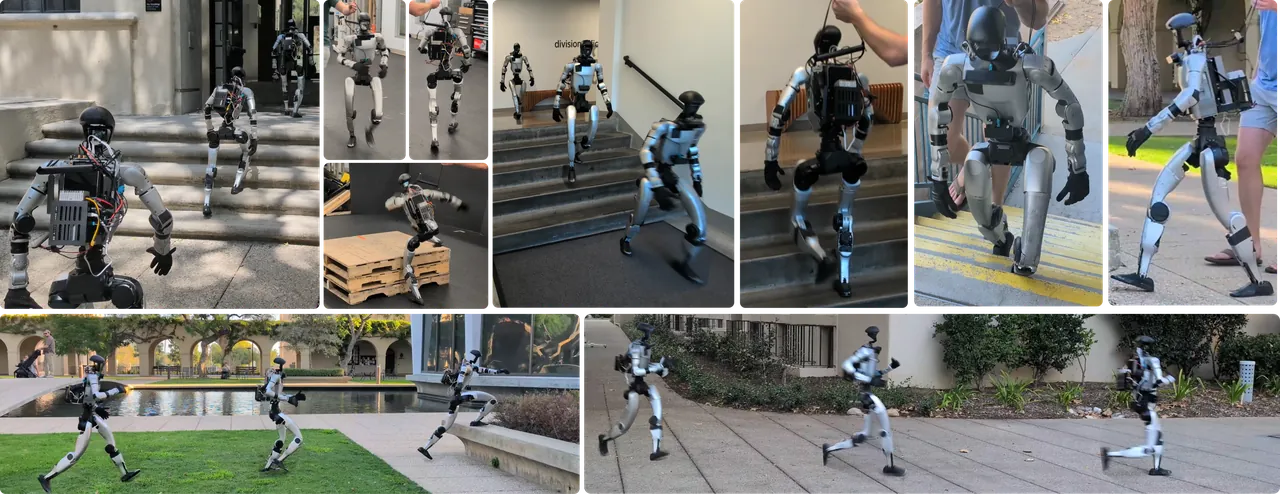
Figure 7: The policy pair on hardware under many conditions. Staircases of differing geometry, straight and turning walking and running on flat ground, and jumps onto several platforms including a running start.
Because the input is raw depth, moving outdoors is easy and needs no adjustment relative to indoors. The hardware results are reported at useful granularity: 15 consecutive stairs climbed without incident; six geometrically distinct real staircases traversed successfully, both up and down; walking and running indoors and outdoors, with transitions onto terrain from both fast and slow states; the bottom-right panel of Figure 7 shows the robot running at 2 m/s while turning along its path; boxes are both jumped onto and jumped off, including with a running start. The authors also specifically report approaching stairs on hardware at 0.8, 1.5, and 2.0 m/s and successfully transitioning onto the terrain. On motion quality, the authors describe hardware motions as smooth, natural, and relatively quiet, especially on terrain such as stairs, where other approaches may slam the foot into the ground. The two-camera policy also deploys in real environments with walls, trees, and shrubs, which suggests that not every perceptive condition has to be simulated.
Two-Camera Ablation: Removing the Upper Camera Drops Box Terrain from 100% to 57.3%
| Terrain type | Both cameras | Lower camera only | Delta |
|---|---|---|---|
| Flat | 100% | 100% | 0 |
| Box | 100% | 57.3% | -42.7 points |
| Stairs up | 82.7% | 71.3% | -11.4 points |
| Stairs down | 97.3% | 88.0% | -9.3 points |
Table 4 (paper Table IV): the effect of the upper camera on in-distribution traversal. Removing it costs up to 43% of success, on box terrain.
Plenty of prior work uses a single downward-facing camera. This paper needs two because it requires the robot to adjust speed before reaching the terrain: at up to 2.5 m/s a downward camera sees the obstacle too late. To isolate the variable, these experiments use only the original pretrained generator (no RL fine-tuning) and train two versions, with and without the upper camera. The results are in Table 4: removing the upper camera costs up to 43% success (box terrain 100% to 57.3%), 11.4 and 9.3 points on stairs up and down respectively, and nothing on flat ground. The authors inspected the box-terrain trajectories and confirmed that the large majority of failures are running straight into the box, and that success falls as speed rises, which is exactly the quantification of "see early, decelerate early."
Limitations
The paper has a dedicated limitations section with three author-stated items. First, RL fine-tuning relies on hand-designed rewards: although these rewards are fairly general, they may not extend to every possible motion. Second, depth-only perception limits the semantics available to the policy, and the example the authors give is concrete: there may be box-shaped objects we do not want the robot to jump onto, and the current method offers no way to encode that. Third, the data pipeline still needs manual tuning: hyperparameters for the transition stage must be hand-set, and selecting human reference motions for optimization is still heuristic or human-driven. The authors say plainly that both data-pipeline limitations must be resolved before the method can scale to arbitrary motions.
The following are my own additions from an engineering and experimental-design standpoint. First, the terrain-consistency rewards depend on a terrain SDF, and an SDF exists only in simulation. Both $r_{pen}$ and $r_{con}$ in Table 2 are built on $\text{sdf}(p)$, so the entire RL fine-tuning signal is simulation-exclusive; "learning from real hardware data" is still future work, which means the improvement on the real robot rests wholly on sim-to-real transfer. The paper offers no direct comparison of whether the gains measured in simulation also appear on hardware, since only the multi-terrain fine-tuned version was deployed and there is no side-by-side footage against the pretrained version. Second, mode labeling was done by a single person. Fifty shuffled rollouts were labeled by one human, with undecidable cases counted as incorrect, but no inter-rater agreement is reported, and correct-mode rate happens to be the paper's most striking number (0% to about 80%). Third, the PPO comparison was stopped early. The authors themselves admit PPO may still have been improving, so "offline beats online" holds at the 2,000-iteration mark and cannot be extrapolated into a claim that PPO's convergence ceiling is lower. Fourth, velocity RMSE is reported on flat ground only. Table 3 is the key evidence for pipeline quality, yet there is no corresponding measurement on terrain, where whether the robot should track the commanded speed at all is deliberately relaxed by the reward. Fifth, the evaluation sample sizes and statistics are light. The two-camera ablation and the velocity evaluation use a handful of rollouts per terrain and 50 per speed respectively; success rates are quoted to a tenth of a point (57.3%, 82.7%) with no confidence intervals, whereas Table 3 does report CIs and Table 4 does not. Sixth, the generator receives no proprioception. The authors compensate with pixel 3D coordinates in a gravity-aligned root frame, which holds while the IMU and state estimation are trustworthy, but it moves the dependence on gravity estimation into the input channels, and the paper does not discuss how state-estimation drift affects the generator.
Summary and Outlook
The three contributions deserve separate verdicts. The architecture (perceptive generator plus CLF-RL tracker, split across 50 Hz and 0.24 s) is not a new paradigm; SONIC and PARC already walked that road. What this paper does is finish it into a deployable form: raw depth input, no odometry, no height map, the same policy pair indoors and outdoors, accurate velocity tracking. The data pipeline (human data to multiple-shooting dynamic optimization to contact ground truth to kinematic retargeting across terrain dimensions to re-optimization to Motion Bricks in-betweening to 10,000 clips over 140 geometries) handles the dirtiest part of the mimic route, and Table 3 shows it is not optional: clip velocity accuracy is the ceiling on final policy velocity accuracy, and using Motion Bricks alone raises fast-band RMSE from 0.442 to 0.896. Offline RL fine-tuning of the generator is the genuinely new piece, and the authors claim it as a first: using RL to fine-tune a perceptive generative model for dynamic, terrain-aware humanoid locomotion. Its cleverness is not in the algorithm, since AWR, FVI, and advantage weighting are all existing components, but in the choice of search space: exploration is moved out of the 2,728-dimensional action space and into the conditioning, the spawn positions, and the flow-matching initial noise, while the tracker is frozen into "part of the robot's dynamics," so MDP steps become 0.24 s re-plans and the horizon shrinks enough for offline methods to cope.
Two lessons are worth stealing if you build humanoid controllers. The first is prefix attention isolation: making the conditioning tokens not attend to the output tokens lets the prefix encoder be cached for faster inference and frozen for critic reuse, so a single structural decision serves both deployment and training. The second is that mode selection has to be fixed in the generator, not the tracker: no matter how accurate the tracker is, it faithfully executes whatever reference it is given, and the decision about which skill clears an obstacle is made at the moment the reference is generated.
The paper lists four directions of future work: improving the search inside generator RL, which would not only raise motion quality but could also generate new motions the way PARC does, provided an efficient structured search can be found; extending the method to learn from real hardware data so it can keep improving from real deployment; on the data side, current human datasets carry no terrain ground truth, so bringing objects and terrain into datasets would make the problem more scalable, alongside better transition generation and new offline terrain-aware motion models; and integrating the controller pair into a navigation autonomy stack with safety and obstacle avoidance woven in, which is what further real deployment requires.