How to Build a Humanoid Robot: A Seven-Layer Constraint Chain from Joint Modules to Sim-to-Real
A humanoid robot is not an assembly of seven modules but a stack of physics equations that set each other's boundary conditions. This article computes the whole-machine stack layer by layer: joint motor modules (declared torque versus real quasi-static CoP demand — BHL's hip has only 0.9x margin) -> IMU (lever-arm pseudo-acceleration is 21,752x the sensor noise floor, so mounting position matters four orders of magnitude more than the datasheet) -> materials and structure (three BOM revisions of AgiBot's X1 as a load-path history: every part entering the closed-chain drivetrain upgraded to 7075-T6 / TC4 / 17-4PH) -> sensors (fix the observation space before the shopping list) -> battery and BMS ('all joints at peak simultaneously' is physically impossible: G1's 46,062 W against a 421 Wh pack is 109 C) -> software control and the CAN-level low-side boards (22 nodes at 500 Hz on one bus is 130.9% load, so it must be split into four) -> simulation training and sim-to-real (9 of 12 real failure modes are hardware calibration, not simulation fidelity). Every figure comes from programmatic parsing of the five machines' public model files plus official vendor specifications, and is recomputable.
Introduction: a humanoid robot is a stack of mutually constraining physics equations
Ask "how do you build a humanoid robot" and nearly every answer lands on one of two extremes. One is launch-event copy ("40 degrees of freedom, two hours of runtime, end-to-end foundation models"); the other is a shopping list ("buy 20 joint modules, one NUC, one IMU"). The first explains where none of the numbers come from. The second explains why these particular numbers.
This article walks the whole-machine technology stack top to bottom: joint motor modules → IMU → materials and structural design → sensors → battery and BMS → software control / drives / the CAN-level low-side boards → simulation training and sim-to-real. Every layer gets the same question: how is this parameter nailed down by the layers above and below it? Because a humanoid is not an assembly of modules, it is a stack of interlocked physics equations. Ankle torque determines how far the centre of pressure can be pushed along the foot; that lever arm determines where the IMU must go; the IMU's lever-arm pseudo-acceleration determines how many orders of magnitude above the sensor noise floor it sits; whole-machine peak power determines how many C the battery pack has to sustain; and the pack's C-rate ceiling in turn decides whether "every joint at peak simultaneously" can physically happen at all.
Two reference sets carry the analysis. The first is a reproducible open-source reference: UC Berkeley's Berkeley Humanoid Lite (BHL, arXiv:2504.17249), 22 DoF and 16.33 kg, with motor part numbers, FOC firmware, 3D-printing parameters and the Isaac Lab training config all public on its official documentation site — the only sample where "follow the instructions and you really can build it" holds. The second is a set of industrial references: Unitree G1 (29 DoF / 35.12 kg), Unitree H1 (10 DoF / 51.65 kg), AgiBot Lingxi X1 (12 DoF in the legs / 35.32 kg) and RoboParty ATOM01 (23 DoF / 33.97 kg). Every torque, velocity, mass and inertia figure comes from programmatic parsing of these machines' public URDF / MJCF files (G1 URDF, H1 URDF, X1 URDF and MJCF, ATOM01 URDF); battery pack parameters come from official vendor specifications; the BMS device stack comes from published TI / ADI / Renesas material; component part numbers and specifications come from the 873 component records already in the RobotWorld knowledge base, each of which can be looked up there with its original specs. Every external link in this article is listed by class in the "Data sources and parsing conventions" section at the end.
This article endorses no vendor and ranks no machine. What it does is lay out the engineering constraints at each layer with numbers you can recompute. Full parsing methodology and data sources are at the end.
The whole-machine stack: seven layers, each one setting the boundary conditions for the next
flowchart TD
 A["1. Joint motor module
frameless motor + reducer + dual encoders + driver
Sets: torque / speed / back-drivability / reflected inertia"]
 B["2. Structure and materials
closed-loop linkage / 7075-T6 / TC4 / 17-4PH
Sets: mass distribution → static torque demand per joint"]
 C["3. IMU
mounting location + lever arm r
Sets: the ceiling on state-estimation accuracy"]
 D["4. Sensors
vision / lidar / 6-axis F-T / tactile / joint encoders
Sets: the policy observation space"]
 E["5. Battery + BMS
series count S / capacity Ah / C-rate ceiling / dual-path current sensing
Sets: deliverable peak power and runtime"]
 F["6. Low-side boards and bus
FOC current loop → CAN topology → onboard compute
Sets: control frequency and the node-count ceiling"]
 G["7. Simulation and sim-to-real
Isaac Lab training → MuJoCo sim2sim → ONNX on the robot
Sets: whether the policy survives real hardware"]
 B --> A
 A --> E
 B --> C
 A --> D
 E --> F
 A --> F
 C --> G
 D --> G
 F --> G
 G -.->|domain randomisation pushes back: hardware must carry margin| A
Layer 1: the joint motor module — settle the torque budget before you talk about what to buy
Joint modules are 40–60% of whole-machine BOM cost, and the reducer inside a single module is 30–50% of that module. This is the most expensive block on the robot and the easiest one to buy wrong. The classic mistake is ordering off peak torque — and peak torque is precisely the least trustworthy field in a URDF.
1.1 The declared-torque landscape across five robots
Multiply effort (peak torque, Nm) by velocity (peak angular velocity, rad/s) for every revolute joint in all five URDFs and sum the products, and you get the theoretical total power of "every joint at peak at the same instant". The results:
| Robot | Mass (kg) | Revolute joints | Σ effort (Nm) | Σ peak power (W) | Nm/kg | W/kg | W/Nm |
|---|---|---|---|---|---|---|---|
| Berkeley Humanoid Lite | 16.33 | 22 | 440 | 6,600 | 26.9 | 404 | 15.00 |
| RoboParty ATOM01 | 33.97 | 23 | 972 | 8,488 | 28.6 | 250 | 8.73 |
| AgiBot Lingxi X1 (legs only) | 35.32 | 12 | 1,320 | 12,800 | 37.4 | 362 | 9.70 |
| Unitree H1 | 51.65 | 10 | 1,880 | 36,720 | 36.4 | 711 | 19.53 |
| Unitree G1 (29 DoF) | 35.12 | 29 | 1,464 | 46,062 | 41.7 | 1,312 | 31.46 |
The last column, W/Nm (watts per newton-metre of torque), is the most informative one in this table. It measures speed design intent, not strength design intent. ATOM01 and X1 both sit at 9–10 W/Nm, meaning their joints are quasi-static, high-torque low-speed designs (X1's hip pitch is only 8 rad/s, about 76 rpm). G1 reaches 31.5, meaning it is designed for dynamic gaits and even running (hip 32 rad/s, ankle 37 rad/s, close to 354 rpm). The same 88 Nm hip joint, paired with 8 rad/s versus 32 rad/s, is a completely different motor and a completely different reduction ratio. That difference propagates all the way down into reducer selection, battery C-rate and bus bandwidth.
({"_height": "420px",
 "backgroundColor": "transparent",
 "grid": {"left": 70, "right": 40, "top": 46, "bottom": 70},
 "tooltip": {"trigger": "axis",
 "axisPointer": {"type": "shadow"},
 "backgroundColor": "rgba(15,23,42,0.95)",
 "borderColor": "#3ddc97",
 "borderWidth": 1,
 "textStyle": {"color": "#e2e8f0"},
 "formatter": function (p) {var d = p[0];
 var extra = {"BHL": "22 joints · Σ440 Nm · 16.33 kg · 26.9 Nm/kg",
 "ATOM01": "23 joints · Σ972 Nm · 33.97 kg · 28.6 Nm/kg",
 "X1 (legs)": "12 joints · Σ1320 Nm · 35.32 kg · 37.4 Nm/kg",
 "H1": "10 joints · Σ1880 Nm · 51.65 kg · 36.4 Nm/kg",
 "G1": "29 joints · Σ1464 Nm · 35.12 kg · 41.7 Nm/kg"};
 return "" + d.name + "
Peak power density: " + d.value + " W/kg
" + (extra[d.name] || "");}},
 "xAxis": {"type": "category",
 "data": ["BHL", "ATOM01", "X1 (legs)", "H1", "G1"],
 "axisLabel": {"color": "#94a3b8", "fontSize": 12},
 "axisLine": {"lineStyle": {"color": "#334155"}}},
 "yAxis": {"type": "log",
 "name": "W/kg (log)",
 "nameTextStyle": {"color": "#94a3b8"},
 "axisLabel": {"color": "#94a3b8"},
 "splitLine": {"lineStyle": {"color": "rgba(148,163,184,0.15)"}}},
 "series": [{"type": "bar",
 "barWidth": "46%",
 "data": [{"value": 404, "itemStyle": {"color": "#3ddc97"}},
 {"value": 250, "itemStyle": {"color": "#4aa8f0"}},
 {"value": 362, "itemStyle": {"color": "#e0b341"}},
 {"value": 711, "itemStyle": {"color": "#f0708a"}},
 {"value": 1312, "itemStyle": {"color": "#9d7bf0"}}],
 "label": {"show": true, "position": "top", "color": "#e2e8f0", "formatter": "{c} W/kg"},
 "markLine": {"symbol": "none",
 "lineStyle": {"color": "#f0708a", "type": "dashed"},
 "label": {"color": "#f0708a", "formatter": "G1 = 3.2× BHL"},
 "data": [{"yAxis": 404}]}}]})
1.2 Declared torque versus real demand: the quasi-static CoP model
effort in a URDF is the vendor's declared peak joint torque. It does not tell you whether that torque is enough, and it does not tell you what operating condition it was sized for. The simplest recomputable model for "enough" is single-leg support, quasi-static, centre of pressure pushed out to the toe: the whole machine mass $m$ is carried by one leg, the CoP moves forward from the ankle axis to the toe, the lever arm is the foot length $L_{foot}$, and the pitch moment the ankle must supply is
$$\tau_{ankle} = m \cdot g \cdot d_{cop}, \qquad d_{cop} \le L_{foot}$$
where $d_{cop}$ is the horizontal distance from the ankle axis to the CoP. $d_{cop} = L_{foot}$ is the worst case (all the weight on the toe, i.e. the instant of push-off or toe-off). Solving backwards gives how far this machine is designed to let the CoP travel:
$$d_{cop}^{max} = \frac{\tau_{ankle}^{declared}}{m \cdot g}$$
Knee and hip are handled by a 2D static balance in a 40° knee-flexed squat (the posture humanoids spend most of their manipulation and disturbance-rejection time in), accumulating thigh, shank and foot masses segment by segment from the URDF link masses and centre-of-mass positions. Results:
| Robot | Foot length (m) | Ankle effort (Nm) | Reachable CoP arm (m) | Share of foot | 40° flex demand: ankle / knee / hip (Nm) | Knee margin | Hip margin |
|---|---|---|---|---|---|---|---|
| ATOM01 | 0.22 | 18 | 0.054 | 39% | 46.7 / 17.6 / 35.9 | 4.5× | 2.2× |
| Unitree H1 | 0.21 | 40 | 0.079 | 58% | 68.4 / 61.9 / 68.4 | 4.9× | 2.9× |
| BHL | 0.22 | 20 | 0.125 | 89% | 22.4 / 6.0 / 21.4 | 3.4× | 0.9× |
| Unitree G1 | 0.17 | 50 | 0.145 | 121% | 41.3 / 25.1 / 14.2 | 5.5× | 6.2× |
| AgiBot X1 | 0.25 | 80 | 0.231 | 144% | 55.4 / 12.5 / 55.4 | 12.0× | 2.7× |
This table yields three hard conclusions, and they are the ones to keep in mind when selecting hardware.
Conclusion one: the ankle is the only genuinely tight joint, and knees are routinely over-designed by 3–12×. All five machines have knee margins ≥3.4×, X1 reaching 12×, while the reachable CoP arm spans 39% to 144% of foot length. ATOM01's ankle is 18 Nm, which means its CoP can never travel past the front 39% of the foot — this machine is physically incapable of a toe-off push and can only walk flat-footed. No software fixes that; it is a hardware ceiling. Conversely, the G1 (121%) and X1 (144%) ankles already exceed what "CoP at the toe" requires, and the surplus is exactly the reserve for dynamic gait: push-off, jumping, landing impact.
Conclusion two: BHL's hip margin is 0.9×, meaning the 21.4 Nm static demand already exceeds the declared 20 Nm. That is deliberate. BHL uses one homogeneous M6C12 motor + 15:1 planetary reduction + a 3D-printed cycloidal disc to build a self-made module (print parameters in the official 3D Printing Instructions), and all 22 joints are 20 Nm @ 15 rad/s — one specification for the whole body. The price is a hip that runs at the edge in a deep squat, with the policy trained to avoid extreme postures. This is a textbook trade between "cheap and reproducible" and "performance margin", and it is written openly into the hardware rather than hidden.
Conclusion three: declared effort is not sized for statics, it is sized for dynamic gait. H1 is the best evidence. Its knee needs 61.9 Nm statically at 40° flexion against a declared 300 Nm effort (4.9× margin); its ankle needs 68.4 Nm against a declared 40 Nm effort (0.58×, undersized). One joint 5× over-provisioned and another 42% under-provisioned on the same machine has exactly one explanation: H1's knee is sized for the swing-phase dynamic acceleration (the $J\dot\omega$ term) of walking, while its ankle is assumed never to carry full weight on the toe — and H1's gait is indeed heel-strike-dominated and flat-footed. That corroborates the ATOM01 39% CoP finding: ankle torque is the fingerprint of gait type.
({"_height": "400px",
 "backgroundColor": "transparent",
 "legend": {"data": ["Knee margin", "Hip margin"], "textStyle": {"color": "#94a3b8"}, "top": 4},
 "grid": {"left": 70, "right": 40, "top": 56, "bottom": 46},
 "tooltip": {"trigger": "axis",
 "axisPointer": {"type": "shadow"},
 "backgroundColor": "rgba(15,23,42,0.95)",
 "borderColor": "#3ddc97",
 "borderWidth": 1,
 "textStyle": {"color": "#e2e8f0"},
 "formatter": function (ps) {var s = "" + ps[0].name + "";
 for (var i = 0; i < ps.length; i++) {s += "
" + ps[i].marker + ps[i].seriesName + ": " + ps[i].value + "×";}
 return s;}},
 "xAxis": {"type": "category",
 "data": ["BHL", "ATOM01", "G1", "H1", "X1"],
 "axisLabel": {"color": "#94a3b8"},
 "axisLine": {"lineStyle": {"color": "#334155"}}},
 "yAxis": {"type": "log",
 "name": "Margin (log)",
 "nameTextStyle": {"color": "#94a3b8"},
 "axisLabel": {"color": "#94a3b8"},
 "splitLine": {"lineStyle": {"color": "rgba(148,163,184,0.15)"}}},
 "series": [{"name": "Knee margin",
 "type": "bar",
 "barWidth": "30%",
 "itemStyle": {"color": "#e0b341"},
 "label": {"show": true, "position": "top", "color": "#e2e8f0", "formatter": "{c}×"},
 "data": [3.36, 4.54, 5.54, 4.85, 12.03],
 "markLine": {"symbol": "none",
 "lineStyle": {"color": "#f0708a", "type": "dashed", "width": 2},
 "label": {"color": "#f0708a", "formatter": "1.0× = exactly enough statically"},
 "data": [{"yAxis": 1.0}]}},
 {"name": "Hip margin",
 "type": "bar",
 "barWidth": "30%",
 "itemStyle": {"color": "#4aa8f0"},
 "label": {"show": true, "position": "top", "color": "#e2e8f0", "formatter": "{c}×"},
 "data": [0.93, 2.23, 6.21, 2.92, 2.71]}]})
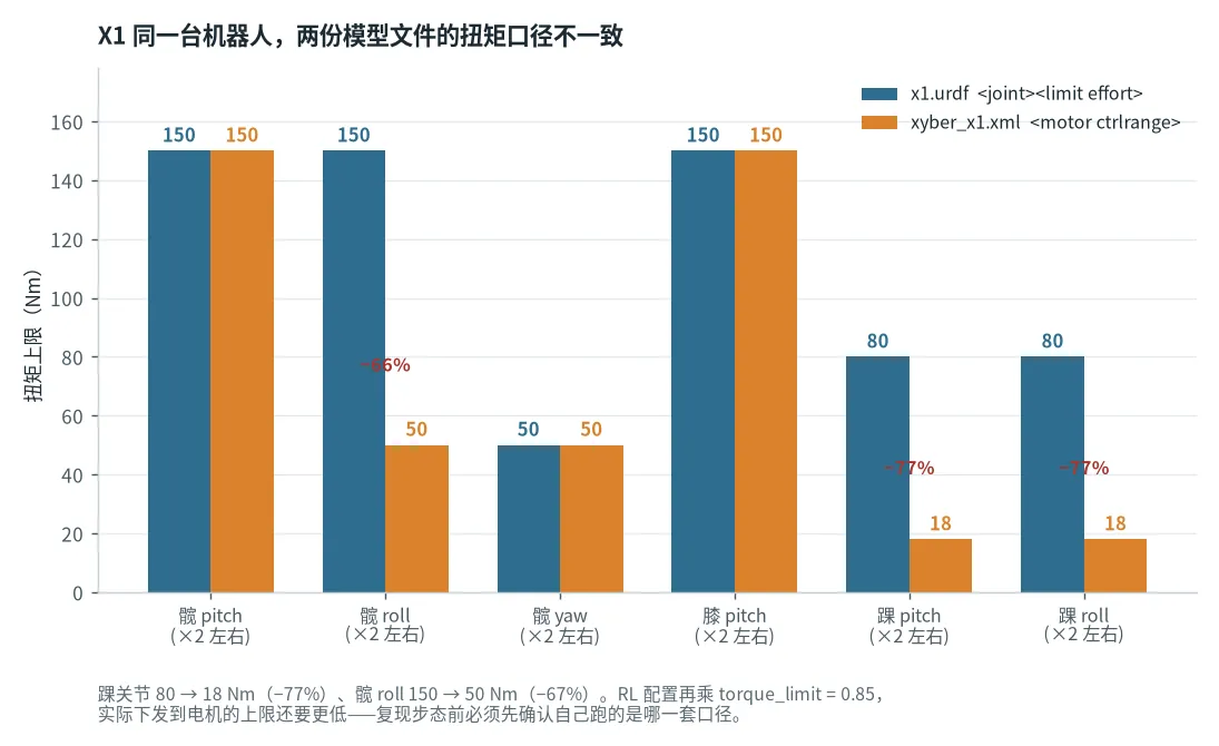
x1.urdf sum to 1320 Nm of effort, while the 12 motors in xyber_x1_serial.xml (MuJoCo) sum to only 872 Nm of ctrlrange — a 51.4% gap. The ankle drops from 80 Nm to 18 Nm (−77%) and hip roll from 150 Nm to 50 Nm (−67%). If you read only one of the two files, every margin you compute for the whole machine can be wrong. Any torque budget must first state which file it was read from.1.3 Inside the module: motor, reducer, encoder and driver are one coupled design
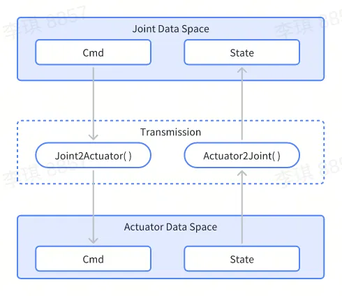
A joint module is not one part, it is four parts designed as a unit: frameless motor (produces torque) + reducer (trades speed for torque) + dual encoders (close the loop) + driver (FOC current loop). Choosing any one of them locks the other three.
Torque amplification and speed loss are a first-order relationship. With reduction ratio $n$, motor torque constant $K_t$ (Nm/A) and rotor inertia $J_r$, the output side is:
$$\tau_{out} = n \cdot \eta \cdot K_t \cdot I, \qquad J_{reflected} = n^2 \cdot J_r, \qquad \omega_{out} = \frac{\omega_{motor}}{n}$$
That $n^2$ term is the central tension in all joint design: double the reduction ratio and torque doubles (good), but the rotor inertia reflected to the output quadruples (bad). More inertia makes a joint "dull" — not back-drivable, low impedance-control bandwidth, and on impact it passes the whole shock into the links. This is precisely why the quasi-direct-drive (QDD) route exists: a small ratio (6–15:1) plus a high-current motor, sacrificing torque density for back-drivability and bandwidth. BHL is pure QDD (15:1 planetary); H1 and X1 hips and knees are also low-ratio planetary; only the small-torque high-bandwidth positions — wrists, dexterous hands — use harmonic drives at 100:1 and above.
BHL's motor characterisation documentation is the most complete public characterisation of a self-built module currently available — the only "bare motor to finished joint" measured dataset you can actually get (module assembly and gearbox fabrication are in Building the Actuator):
| Parameter | T-Motor M6C12 (BHL primary) | T-Motor 5010-110KV (alternate) | Notes |
|---|---|---|---|
| Phase resistance R | 0.1886 Ω | 0.6193 Ω | Line-to-line measurement halved; sets copper loss $I^2R$ |
| Phase inductance L | 0.0325 mH | 0.0850 mH | Sets the current-loop bandwidth ceiling $f_c \approx R/2\pi L$ |
| Torque constant $K_t$ (measured) | 0.0919 Nm/A | 0.1176 Nm/A | Derived from $K_t = 11.6955/K_V$ (delta connection) |
| $K_V$ measured vs datasheet | 127.19 vs 150 (−15%) | 99.44 vs 110 (−9.6%) | Datasheet values run systematically high; you must measure them |
| Rotor inertia $J_r$ | 9.942×10⁻⁵ kg·m² | 3.301×10⁻⁵ kg·m² | Reflected after 15:1 → 0.0224 / 0.00743 kg·m² |
| Output Nm/A after reduction | 1.378 (20 Nm needs 14.5 A) | 1.764 (20 Nm needs 11.3 A) | ODRI 4004-300KV×9 gives only 0.351 → 57 A |
| Position encoder | AS5600 magnetic (series resistor added to raise resolution) | same | Magnet glued to the rotor shaft; one I²C read takes 78 µs |
That 78 µs in the last row is an instructive number. BHL reads the AS5600 over I²C, one read costs 78 µs, and that alone puts the position-loop frequency ceiling at about 12.8 kHz — while its firmware runs on a 160 MHz MCU compiled with -O2 (Recoil FOC). In other words, in this design what limits control frequency is not compute, it is the physical transmission time of the encoder interface. Switch to SPI, or replace the magnetic encoder with an incremental one plus interrupt counting, and the same MCU gains an order of magnitude on the loop. This is the most typical trap in the "drives / low-side boards" layer: budget the interface before you budget the compute.
Likewise, a datasheet $K_V$ that runs 15% high means a current limit designed straight off the datasheet $K_t$ is 15% wrong: you think 14.5 A gives 20 Nm and actually get 17 Nm, or you drive 17 A to reach 20 Nm and blow past the driver's thermal design. BHL's practice is to run a locked-rotor / no-load characterisation on every motor before first power-up and write the measured R, L and $K_t$ into the firmware parameter table. Any serious module programme should have this step.
1.4 Reflected inertia: distal joints are motor-dominated, proximal joints are link-dominated
Take the inertia of every link downstream of each BHL joint (folded onto that joint's axis with the parallel-axis theorem, with inputs from the mass / inertia / origin fields of the official URDF), and divide it by the reflected rotor inertia $n^2 J_r = 0.0224$ kg·m². The resulting table decides how each joint has to be controlled:
| Joint | Downstream link inertia (kg·m²) | Reflected rotor inertia (kg·m²) | Ratio (rotor/link) | Dominated by | Control implication |
|---|---|---|---|---|---|
| Elbow roll | 0.00022 | 0.0224 | 103× | Motor | Almost pure rotor inertia, hard to back-drive, needs impedance/admittance control |
| Ankle roll | 0.00098 | 0.0224 | 22.8× | Motor | A contact joint that is nonetheless motor-dominated → landing impact is absorbed entirely by the current loop |
| Shoulder yaw | 0.00082 | 0.0224 | 27.2× | Motor | Small link + high ratio, textbook motor-dominated |
| Ankle pitch | 0.00765 | 0.0224 | 2.9× | Motor | Transition region |
| Elbow pitch | 0.01276 | 0.0224 | 1.8× | Motor | Transition region |
| Knee pitch | 0.05608 | 0.0224 | 0.4× | Link | Link-dominated, back-drivable, direct force control works |
| Shoulder pitch / roll | 0.068 / 0.073 | 0.0224 | 0.3× | Link | Link-dominated |
| Hip yaw | 0.08021 | 0.0224 | 0.3× | Link | Link-dominated |
| Hip pitch | 0.18273 | 0.0224 | 0.1× | Link | Purely link-dominated, rotor inertia negligible |
| Hip roll | 0.19930 | 0.0224 | 0.1× | Link | Purely link-dominated |
({"_height": "440px",
 "backgroundColor": "transparent",
 "grid": {"left": 130, "right": 70, "top": 30, "bottom": 50},
 "tooltip": {"trigger": "axis",
 "axisPointer": {"type": "shadow"},
 "backgroundColor": "rgba(15,23,42,0.95)",
 "borderColor": "#9d7bf0",
 "borderWidth": 1,
 "textStyle": {"color": "#e2e8f0"},
 "formatter": function (p) {var d = p[0];
 return "" + d.name + "
Rotor/link inertia ratio: " + d.value + "×
" +
 (d.value > 1? "Motor-dominated → poor back-drivability, needs impedance control": "Link-dominated → back-drivable, direct force control");}},
 "xAxis": {"type": "log",
 "name": "Ratio (log)",
 "nameTextStyle": {"color": "#94a3b8"},
 "axisLabel": {"color": "#94a3b8"},
 "splitLine": {"lineStyle": {"color": "rgba(148,163,184,0.15)"}}},
 "yAxis": {"type": "category",
 "data": ["Hip roll", "Hip pitch", "Shoulder roll", "Shoulder pitch", "Hip yaw", "Knee pitch", "Elbow pitch", "Ankle pitch", "Ankle roll", "Shoulder yaw", "Elbow roll"],
 "axisLabel": {"color": "#94a3b8", "fontSize": 12},
 "axisLine": {"lineStyle": {"color": "#334155"}}},
 "series": [{"type": "bar",
 "barWidth": "55%",
 "data": [{"value": 0.11, "itemStyle": {"color": "#3ddc97"}},
 {"value": 0.12, "itemStyle": {"color": "#3ddc97"}},
 {"value": 0.31, "itemStyle": {"color": "#3ddc97"}},
 {"value": 0.33, "itemStyle": {"color": "#3ddc97"}},
 {"value": 0.28, "itemStyle": {"color": "#3ddc97"}},
 {"value": 0.4, "itemStyle": {"color": "#3ddc97"}},
 {"value": 1.76, "itemStyle": {"color": "#e0b341"}},
 {"value": 2.93, "itemStyle": {"color": "#e0b341"}},
 {"value": 22.8, "itemStyle": {"color": "#f0708a"}},
 {"value": 27.3, "itemStyle": {"color": "#f0708a"}},
 {"value": 103.4, "itemStyle": {"color": "#f0708a"}}],
 "label": {"show": true, "position": "right", "color": "#e2e8f0", "formatter": "{c}×"},
 "markLine": {"symbol": "none",
 "lineStyle": {"color": "#94a3b8", "type": "dashed", "width": 2},
 "label": {"color": "#94a3b8", "formatter": "1.0× boundary"},
 "data": [{"xAxis": 1.0}]}}]})
This chart is why "one set of PD gains for the whole body" is guaranteed to fail on real hardware. The hip's rotor inertia is only 10% of what is downstream of it, so a torque command moves the links immediately; elbow roll's rotor inertia is 103× the link inertia, so the torque you send goes into accelerating the rotor and the link barely moves. G1's legged_gym config groups exactly this way: hip $K_p=100$, knee $K_p=150$, ankle $K_p=40$ Nm/rad, with damping hip 2 / knee 4 / ankle 2. The knee gets the highest stiffness because it is link-dominated and must hold 61.9 Nm of static moment; the ankle gets the lowest because it is motor-dominated and is a contact joint, where stiffness would drive ground impact straight into the base.
1.5 Reducer and module selection: the real shelf in the knowledge base
Translated into procurement language, the constraints above map onto four families of transmission, each with its own territory:
| Type | Typical ratio | Backlash | Back-drivability | Where it goes | Representative parts in the knowledge base |
|---|---|---|---|---|---|
| Planetary (QDD) | 6–48:1 | 10–15 arcmin | Good | Hip, knee, ankle, shoulder — anywhere needing impact absorption and force control | CubeMars AKH70-48 (48:1, 74/222 Nm, 159 Nm/kg, ¥4,888); BHL's self-made 15:1 cycloidal disc |
| Harmonic (strain wave) | 50–160:1 | ≤10 arcsec | Poor (not back-drivable) | Wrist, waist yaw, fingers — low torque, high precision | Harmonic Drive CSD-2A (50–160:1, peak 12–823 Nm); Leaderdrive LHD ultra-thin hollow shaft (axial length ~50% shorter than LHS); Laifual FS series |
| Cycloidal / RV | 27–192:1 | <1 arcmin | Poor | Industrial base and shoulder axes, withstands 5× rated shock; rare on humanoids (too heavy) | Nabtesco RV-E/RV-C (rated 72–4900 Nm, 5× instantaneous shock); Shuanghuan SHPR-E |
| Planetary roller screw (linear) | By lead | — | Medium | Linear hip / knee / ankle (the Optimus route) | Ewellix / Schaeffler (diameter 8–240 mm, lead 2–50 mm, linear speed ≤1.8 m/s, acceleration ≤12,000 rad/s²); Rollvis RV/HRV |
Only three criteria actually matter in selection. First, look at back-drivability before torque density. Put a harmonic drive on a contact joint (ankle) or on any joint that needs force control (knee, shoulder) and you permanently lose the ability to push the robot around by hand; you also lose all mechanical compliance, so every impact is taken by the current loop and the links. Second, harmonic drives hate being dropped. The flexspline is a thin-walled elastic element and a single drop impact can permanently deform it — a real risk during whole-machine bring-up, which is why the industry mainstream puts harmonic drives at the distal arm (where they will not be hit) rather than in the legs. Third, read torque density together with mass. CubeMars AKH70-48's 159 Nm/kg is computed from peak torque; the rated figure is only 74 Nm at 1396 g, i.e. a rated density of 53 Nm/kg. Vendor peak torques are usually 3-second values, so the continuous operating point must be computed from rated specs or you will badly overestimate the module's sustained capability.
Integrated joint modules are already a mature off-the-shelf category, and you can match them directly against whole-machine demand:
| Module | Rated / peak torque | Mass | Supply | Encoder | Bus | Notes |
|---|---|---|---|---|---|---|
| UBTech-style BM series (M5–M200) | 5.5–60 / 12–200 Nm | 280–4700 g | 24/42/72 VDC | Dual 14-bit absolute, position memory across power loss | CAN 1 Mbps | Covers every tier of the body in one family |
| RealMan WHG series | 10–360 Nm | 0.8–5.77 kg | 24/48 V | 16-bit incremental + 18-bit absolute | CAN FD | Electromagnetic brake included, ratios 100/160 |
| Magic Atom H70 | 30 / 96 Nm | 900 g | 48 V | — | CAN / EtherCAT | φ70×96 mm, 12 mm hollow shaft, 30 rpm |
| CubeMars AKH70-48 | 74 / 222 Nm | 1396 g | 48 V (rated 6 A / peak 18 A) | Dual 21-bit magnetic | Dual CAN | Planetary 48:1, 12 arcmin backlash, integrated FOC |
| Wonik Allegro Hand V4 (hand) | 0.70 Nm/joint | 1.08 kg/whole hand | 24 V / 100 W | Potentiometer 0.002° | CAN 333 Hz | 16-joint torque control, 1:369 reduction |
The one thing in that table worth calling out separately is that "position memory across power loss" and "electromagnetic brake" are not options. The moment a humanoid loses power, any joint without a multi-turn absolute encoder or a brake will collapse under gravity — and when a 16–52 kg machine folds from a standing posture, the first thing damaged is precisely the most expensive harmonic drive on it. A multi-turn absolute encoder (e.g. Tamagawa SA series, 17–27 bit per turn + 16 bit multi-turn, battery-less variant TS5966N) guarantees the posture is known at power-up; a brake guarantees hip and knee can hold their own weight when unpowered. Both cost far less than one dropped robot.
Layer 2: the IMU — mounting location matters four orders of magnitude more than device spec
The IMU is the only sensor on a humanoid where mounting it in the wrong place invalidates the whole machine. The reason is not insufficient precision; it is the lever-arm effect. An IMU measures the acceleration at the point where it sits, while the state estimator wants the acceleration of the base centre of mass, and the two differ by terms produced entirely by angular motion.
Let the IMU mounting point $P$ have position vector $\vec r$ relative to the base reference point $O$. The relationship between the two accelerations is the rigid-body kinematics identity:
$$\vec a_P = \vec a_O + \dot{\vec\omega} \times \vec r + \vec\omega \times (\vec\omega \times \vec r)$$
The second term is tangential (angular acceleration × lever arm); the third is centripetal (angular velocity squared × lever arm). Both mix into the same reading as gravity and true translational acceleration, and the estimator cannot separate them. Their magnitude is set entirely by $\vec r$ — and $\vec r$ is a mounting position you picked off-hand on a structure drawing.
2.1 Running the numbers on BHL's real mounting position
BHL's URDF explicitly declares an imu joint (type="fixed", parent = base) at xyz = (0.061722, 0, 0.68). The IMU sits inside the torso, 6.17 cm forward of the base origin and 68 cm above it. Its distance to the torso centre of mass is only 0.065 m, but the lever arm to the ankle joint / base origin is 0.683 m in pitch and 0.0617 m in yaw — a factor of 11 apart.
Plugging in typical walking and disturbance-rejection angular motion:
| Condition | Angular accel. $\dot\omega$ (rad/s²) | Angular vel. $\omega$ (rad/s) | Lever-arm direction | Tangential term (m/s²) | Centripetal term (m/s²) | Combined pseudo-acceleration | Multiple of the BNO085 noise floor |
|---|---|---|---|---|---|---|---|
| Slow turn | 20 | 3 | Pitch r=0.683 m | 13.66 | 6.15 | 14.98 m/s² = 1.53 g | 8,701× |
| Yaw r=0.0617 m | 1.23 | 0.56 | 1.35 m/s² = 0.14 g | 786× | |||
| Fast turn / disturbance | 50 | 6 | Pitch r=0.683 m | 34.15 | 24.59 | 42.08 m/s² = 4.29 g | 21,752× |
| Yaw r=0.0617 m | 3.08 | 2.22 | 3.80 m/s² = 0.39 g | 1,965× | |||
| Fall / landing impact | 100 | 10 | Pitch r=0.683 m | 68.30 | 68.30 | 96.59 m/s² = 9.85 g | 43,503× |
| Yaw r=0.0617 m | 6.17 | 6.17 | 8.73 m/s² = 0.89 g | 3,930× |
Put that table next to device specifications and the conclusion writes itself. The BNO085 accelerometer has an RMS noise of 0.00157 m/s²; the IM10A is 0.00736 m/s². BHL's 0.683 m pitch lever arm generates 34.15 m/s² of tangential pseudo-acceleration in the fast-turn case — 21,752× the BNO085 noise floor, and 43,503× in the fall case.
Device noise is entirely irrelevant at this scale. Paying ten times as much to cut accelerometer noise from 1.57 mg to 0.16 mg buys a 0.015% improvement; moving the IMU from the top of the torso (0.683 m) to the centre of the pelvis (0.1 m) cuts pseudo-acceleration by 85% outright. This is why every humanoid — Unitree, Tesla, Figure, Agility — mounts its IMU in the pelvis or lower torso near the centre of mass rather than in the head or upper chest. The head offers good vision, good cooling and easy assembly, but it has the longest lever arm and is the worst IMU position on the robot.
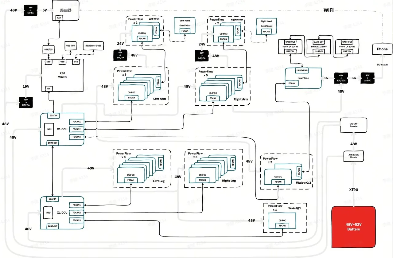
2.2 Why lever-arm pseudo-acceleration is compensable and noise is not
The lever-arm effect has one crucial property: it is deterministic. Given $\vec r$ and $\vec\omega, \dot{\vec\omega}$ (which the gyroscope provides directly), both terms can be subtracted exactly:
$$\vec a_O = \vec a_P - \dot{\vec\omega} \times \vec r - \vec\omega \times (\vec\omega \times \vec r)$$
This is precisely why BHL declares the imu joint coordinates explicitly in its URDF — that xyz=(0.061722, 0, 0.68) is not for rendering, it is for the state estimator's lever-arm compensation. The IMU frame in simulation and the physical mounting position on the robot must match to the millimetre. Both the URDF and the MJCF model imu as a first-class element. Otherwise the base acceleration the policy sees during sim-to-real carries a systematic bias that only appears during angular motion (standing still reveals nothing at all) — one of the hardest classes of bug to diagnose.
Device noise, by contrast, is random. It can only be pushed down by filtering and integration time, never removed. So the priority order for choosing an IMU is: ① mounting position (lever arm, magnitude 10³–10⁴) → ② bias stability (sets long-term drift) → ③ bandwidth (sets whether it can follow impacts above 100 Hz) → ④ RMS noise (magnitude 10⁰). Most selection discussions get this order exactly backwards.
2.3 Device tiers and what is on the shelf
| Parameter | BNO085 (consumer, BHL early) | IM10A (BHL current recommendation) | Xsens MTi-620 (industrial VRU) | Huayi IMU3000 (navigation grade) |
|---|---|---|---|---|
| Accelerometer range | ±16 g | ±16 g | — | ±4 g |
| Accelerometer resolution | 1 mg/LSB | 0.5 mg/LSB | — | — |
| Accelerometer RMS noise | 0.16 mg | 0.75–1 mg | — | Bias instability ≤0.015 mg |
| Accelerometer bias drift | ±150 mg | ±20–40 mg | — | Bias stability ≤0.05 mg |
| Gyro range | ±2000 °/s | ±2000 °/s | 2000 °/s | ±250 °/s |
| Gyro RMS noise | 0.014 °/s | 0.028–0.07 °/s | 0.007 °/s/√Hz | ARW 0.15 °/√hr |
| Gyro bias | ±1 °/s | ±0.5–1 °/s | in-run bias stability 8 °/h | Bias instability ≤0.8 °/h |
| Bandwidth | 8–1000 Hz | 5–256 Hz | Up to 2 kHz output | 200 Hz |
| Magnetometer | ±13 Gauss | ±2 Gauss | Yes (with barometer) | — (GNSS-aided) |
| Interface | I²C / SPI | Direct USB | UART / CAN / RS232 | — |
| Mass / dimensions | — | — | 8.9 g / 28×31.5×13 mm | 22×22×5 mm |
| Positioning | Prototype validation | First choice for open-source humanoids | Industrial / research | Automotive navigation (ASIL-B) |
There is a counter-intuitive fact in this table: when BHL moved from the BNO085 to the IM10A, the noise figures got worse (RMS 0.16 mg → 0.75–1 mg, gyro noise 0.014 → 0.028–0.07 °/s) while bias drift improved dramatically (accelerometer ±150 mg → ±20–40 mg). The reason BHL's IMU comparison documentation gives is purely engineering: the IM10A connects over USB directly, with no Arduino Nano in between, removing one protocol stack layer and one packet-loss source. For state estimation, bias stability matters far more than RMS noise — noise averages away under filtering ($\propto 1/\sqrt{N}$), whereas bias is a systematic error that becomes velocity drift after one integration and position drift after two. A humanoid uses its IMU for attitude and contact detection, not for absolute positioning, so "low drift + a simple reliable data link" beats "low noise + a complex link".
One more easily overlooked issue is range. In the fall case the lever-arm pseudo-acceleration alone reaches 9.85 g; add the real impact and the total reading easily exceeds a ±16 g range. Once the accelerometer clips, attitude estimation diverges immediately — and it happens exactly at the moment attitude estimation is needed most. So size the IMU range against "lever-arm pseudo-acceleration + impact + gravity", not against the walking case. Navigation-grade devices (the Huayi IMU3000 offers only ±4 g) will clip outright in these impact scenarios: they are specified for the steady carriers of cars and drones, not for bipeds that fall over.
Layer 3: materials and structural design — the material migration in a BOM is a history of load paths
Structural design has exactly one central tension: whole-machine mass $m$ appears simultaneously in the numerator of torque demand ($m g d$) and of the runtime budget ($E/P$), and inside inertia ($J \propto m r^2$). Removing 1 kg from the distal leg lowers the static moment demand at ankle, knee and hip, lowers downstream link inertia and lowers whole-machine power draw — three wins at once. Removing 1 kg from the torso lowers only power draw and total static moment, and does almost nothing for inertia (the torso is near the rotation axis, so $r$ is small). Weight reduction therefore always prioritises distal over proximal: every gram in the foot costs more than every gram in the chest.
3.1 The material record across X1's three BOM revisions: upgrades are not random
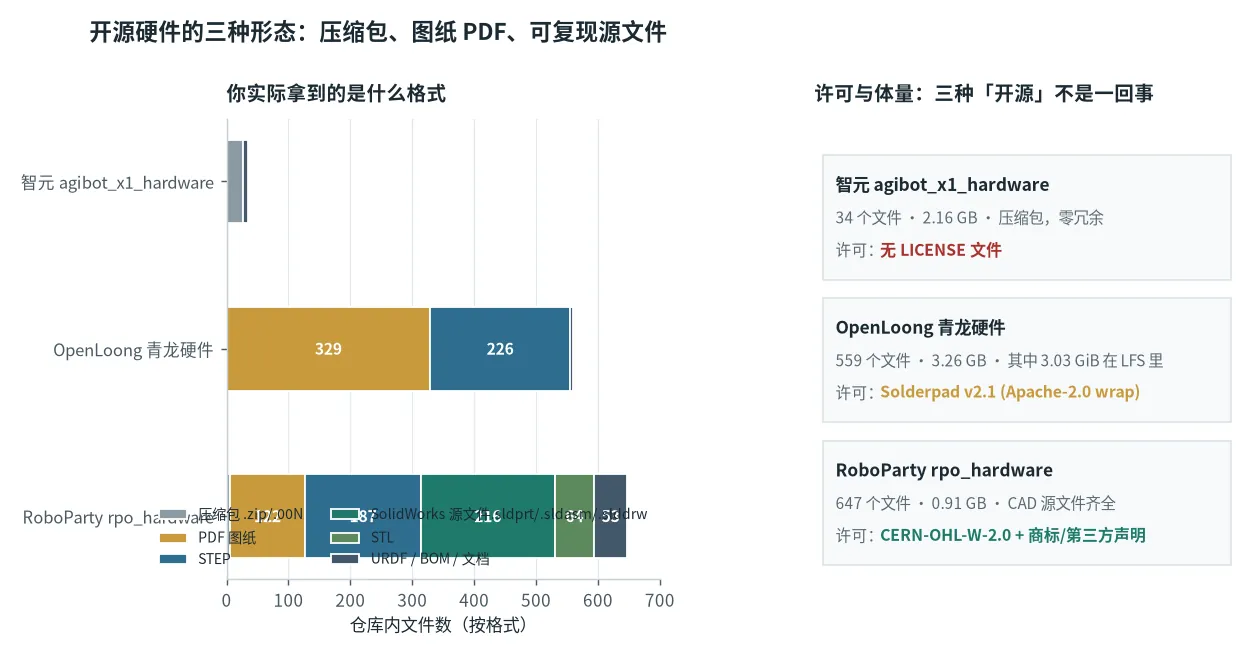
AgiBot X1's hardware repository is the only machine with all three BOM revisions public (agibot_x1_hardware splits them by date: AgiBot X1_20241024 / _20250108 / _20250307, each with a master BOM xlsx, STEP drawings and an assembly SOP; first revision 2024-10-24, third 2025-03-07). ⚠️ That repository has no LICENSE file, so copyright defaults to "all rights reserved" — it can be consulted but not redistributed; by contrast BHL (MIT + CC BY-SA 4.0) and ATOM01 (GPL-3.0) are unambiguous. Reconciling them row by row shows one complete materials iteration:
| Dimension | First BOM (2024-10-24) | Third BOM (2025-03-07) | What the change means |
|---|---|---|---|
| Distinct material annotations | 6 | 11 | From "use whatever is available" to "select by load" |
| Rows carrying a material annotation | 100 | 167 | Material went from optional to a mandatory field |
| 6061-T6 aluminium | 50 instances | Sharply reduced | Replaced by 7075-T6 / 17-4PH |
| 3D-printed resin / ABS | 43 instances | Retained at non-load-bearing positions | Prototype parts promoted to shells and brackets |
| Wrist cross shaft | 40Cr | 17-4PH | Precipitation-hardening stainless: alternating load + corrosion resistance |
| Waist support cross | 6061 | 17-4PH | The core load-bearing part of the closed-loop mechanism |
| Ankle swing arm / foot support / waist linkage | 6061 | 7075-T6 | Yield strength 276 → 503 MPa (+82%) |
| Waist linkage-5 / ankle linkage | 6061 / "titanium alloy" (no grade) | TC4 (Ti-6Al-4V) | Highest specific strength, used at the hardest place to save weight |
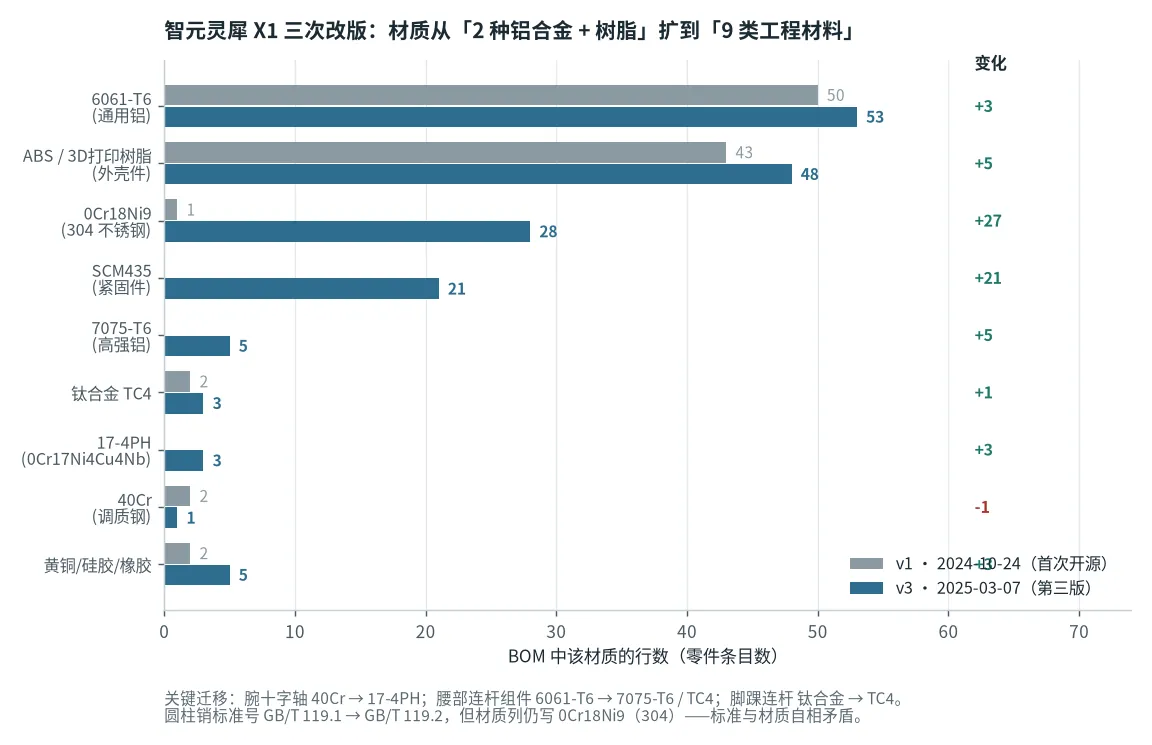
The engineering logic behind this is worth expanding, because every self-designed structure has to walk the same path. The problem with 6061-T6 is not strength, it is fatigue and contact stress. A 276 MPa yield is entirely adequate for a one-off static load, but the pins of a closed-loop linkage see fretting wear plus alternating contact stress — two surfaces sliding microscopically against each other under high pressure, the worst possible duty for aluminium alloy, which initiates fatigue cracks at stresses far below yield. Switching to 17-4PH (precipitation-hardening stainless, 1170 MPa yield after H900 ageing) or 7075-T6 (503 MPa yield) raises fatigue limit and surface hardness together. TC4 goes into the waist linkage because that position demands both high strength and low mass, and TC4's density is only 4.43 g/cm³ (7075 is 2.81, steel is 7.85) — the highest specific strength available, at the cost of difficult machining, high price and poor thermal conductivity.
3.2 The cost structure of three manufacturing routes
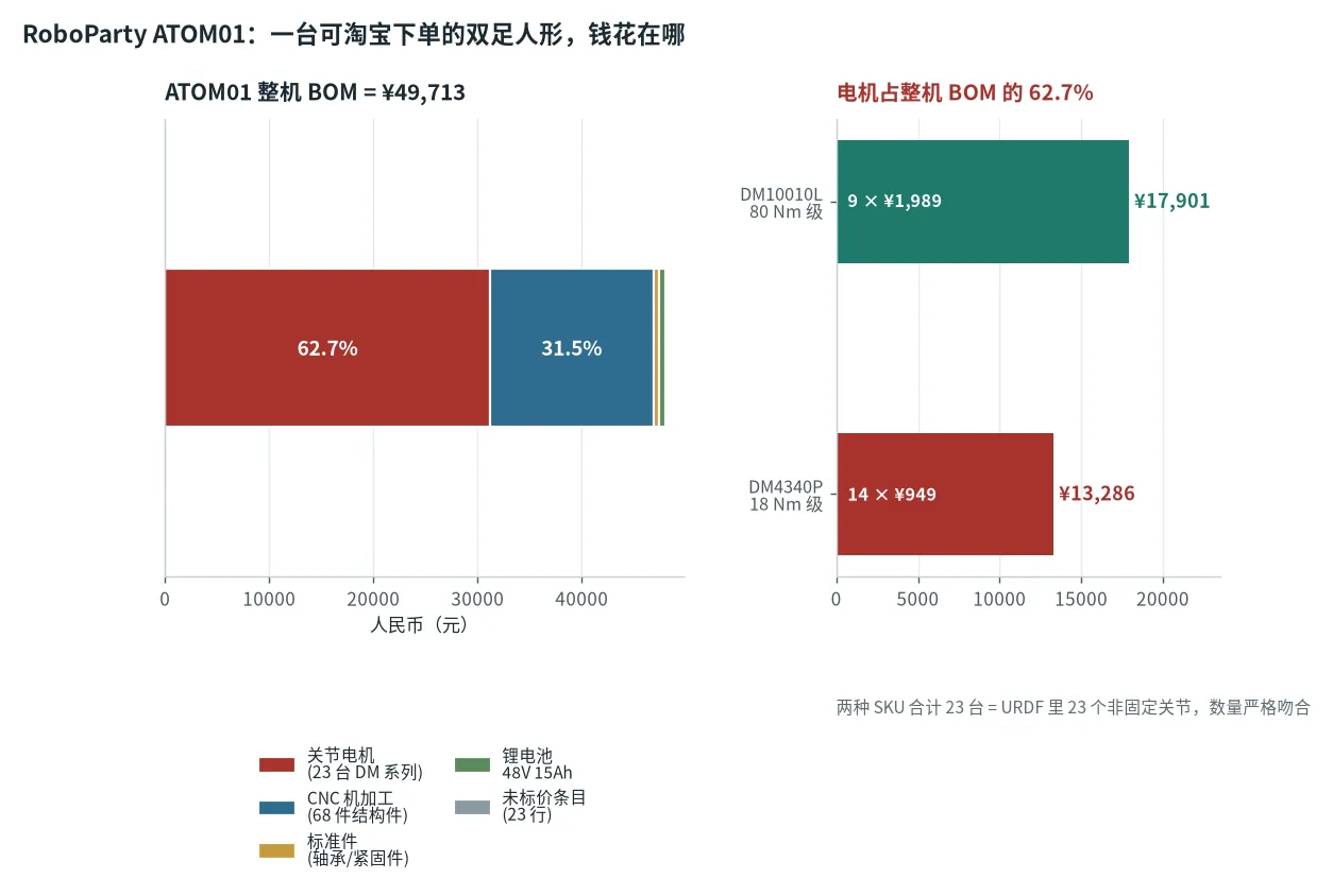
ATOM01 is the only whole machine with complete BOM unit prices public (parts-list xlsx, published alongside the CNC machining and 3D printing drawing sets), and its cost structure gives the real price distribution of the "open-source reproduction" route:
| Cost item | Amount (¥) | Share | Notes |
|---|---|---|---|
| Motors (23 DM series) | 31,187 | 62.7% | 9 × DM10010L (80 Nm tier) + 14 × DM4340P (18 Nm tier) |
| CNC machining (68 parts) | 15,670 | 31.5% | All-metal structure, ¥230 average per part |
| Sensing + compute + battery + cable + fasteners | ~2,850 | 5.8% | Five categories combined, under one tenth of the motors |
| Total | ≈49,700 | 100% | The sheet carries three inconsistent totals (49,713 / 49,743.53 / 49,652.53), a ¥91 = 0.18% spread |
94% of the money goes to motors and CNC. That number completely changes where optimisation effort should go. To cut cost, reducing sensors, switching to a cheaper IMU and using a domestic compute board add up to at most 6% of headroom; there are only two real levers — lower motor unit price (switch to domestic modules or self-built QDD) and lower CNC part count (replace some structural parts with 3D printing or casting). BHL takes exactly the second route: all 22 joints use 3D-printed cycloidal discs plus off-the-shelf T-Motor motors in self-built modules, structural parts are mostly PLA printed on a Bambu Lab X1C, and whole-machine cost drops to a fraction of ATOM01's. The price is the 0.9× hip margin computed earlier.
3.3 Three hidden constraints in structural design
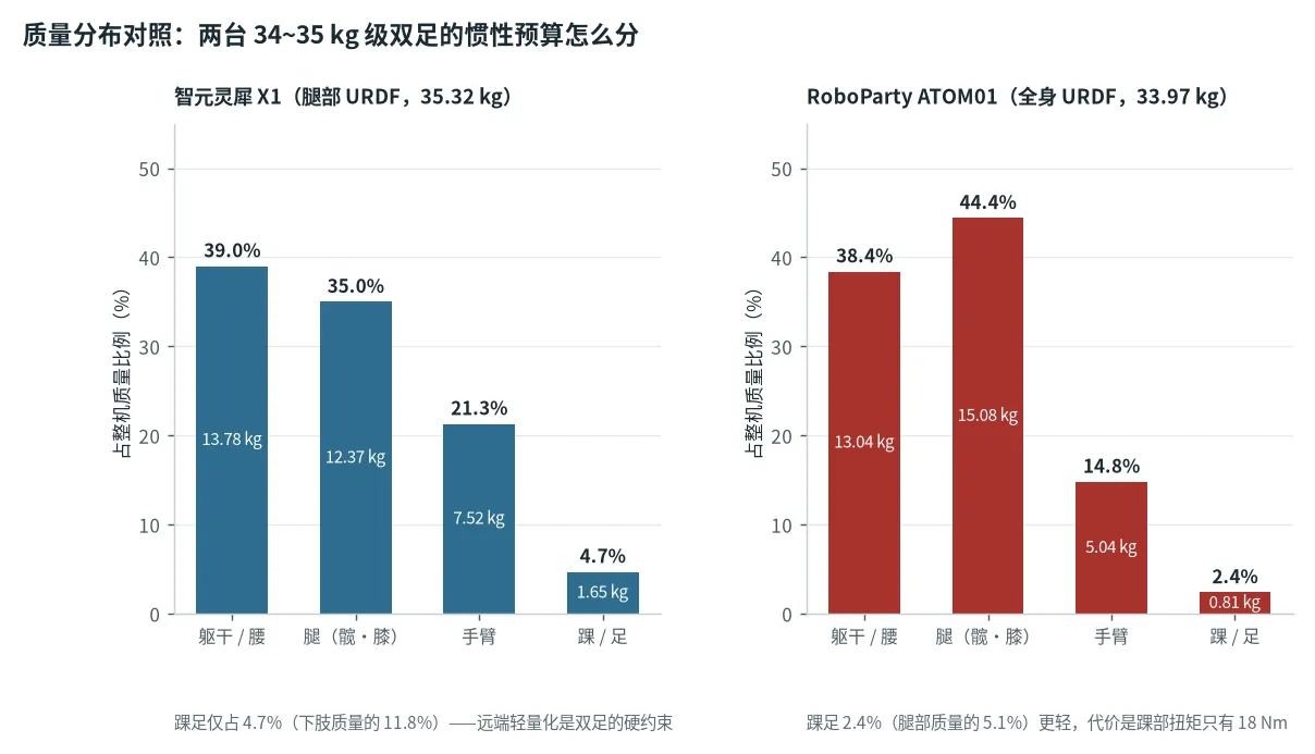
Constraint one: collision geometry is not optional. Only 3 of the 58 links in X1's URDF carry collision geometry (3/58). In simulation this means self-collision detection is effectively off — an arm can pass through the torso, a foot can pass through the shank. A policy trained in that simulation will, on real hardware, do the first thing it was never penalised for: hit its own body. When reproducing, you must add collision geometry yourself, which requires knowing each link's true envelope, which requires the CAD. A URDF without collision bodies is not a "simplified model", it is a physically invalid one.
Constraint two: left-right symmetric parts cannot have their inertia copied. X1's left-wrist link inertia was copied from the right wrist with the mirror sign never flipped (the products of inertia $I_{xy}, I_{yz}$ must change sign). The consequence is nearly invisible in simulation because wrist inertia is a tiny share of the total, but it exposes a general problem: a mirrored part is a geometric mirror in CAD and must be a sign mirror of the inertia tensor in URDF. This is the step most likely to go wrong in a batch export, and the one a self-designed structure must validate with a script.
Constraint three: the harness is the cheapest and the most easily broken part. In industry BOMs the harness is the cheapest line, and it is also the line with the highest flex-fatigue risk (ATOM01 publishes a dedicated harness-routing PDF for it). A humanoid has around 30 moving joints, and at every one of them the harness must follow the full joint travel, bending and twisting repeatedly. BHL's BOM and harness list gives an open-source-grade concrete recipe: 14 AWG silicone wire for power (white/red positive, black ground), 30 AWG for CAN signals, XT60 on the trunk, XT30 on branches, WAGO quick-connects at debug nodes, and a USB-CAN adapter on the host side. Power and signal are routed separately at separate gauges because FOC phase current is high-frequency PWM chopping, which generates common-mode interference on a CAN differential pair. Bundling 14 AWG power and 30 AWG CAN into one loom through the same joint is the most common physical cause of intermittent CAN frame loss.
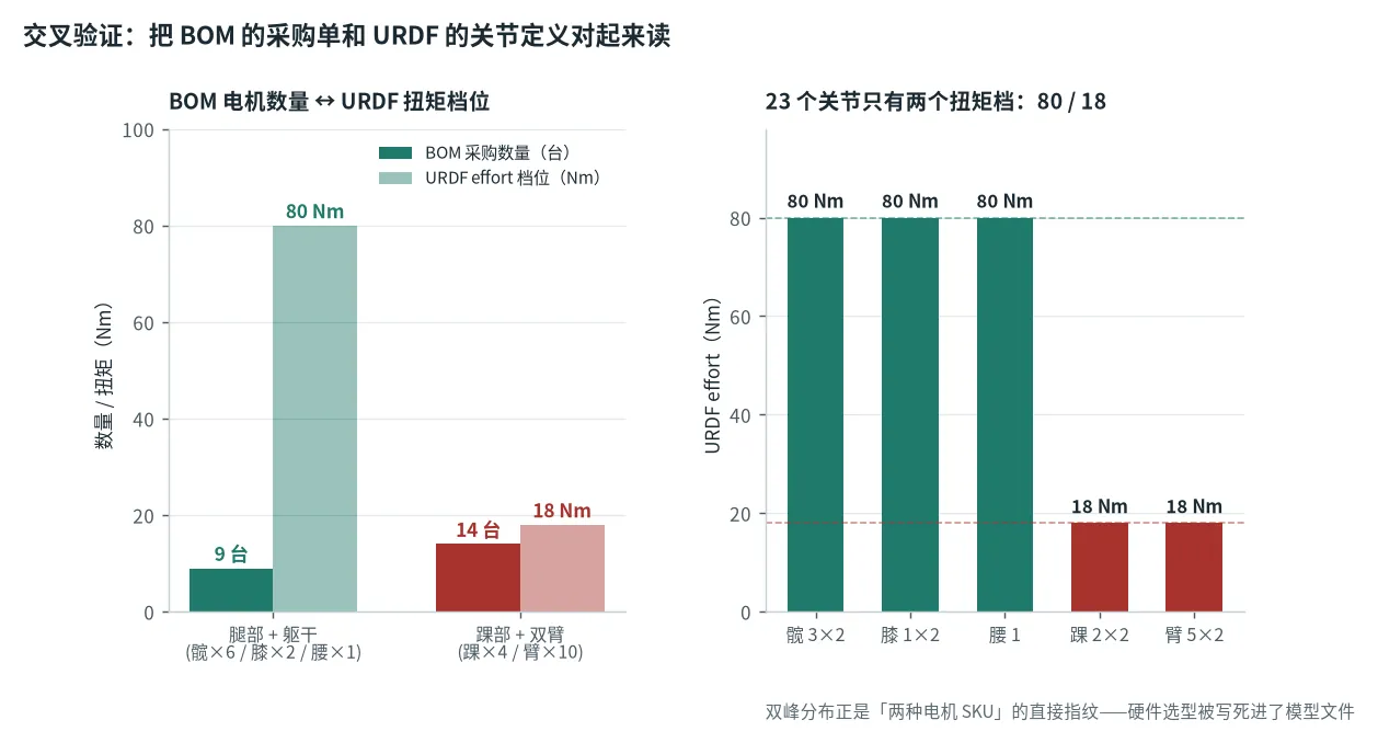
fixed in the URDF. This is not an error, it is a signal: the URDF X1 published is a "leg-gait training model", not a whole-machine model. Training an arm manipulation policy on it will get you nowhere.3.4 A material-selection criteria table
| Position | Dominant load | Recommended material | Why | Avoid |
|---|---|---|---|---|
| Foot / ankle swing arm | Impact + contact stress + wear | 7075-T6 / TC4 with surface hardening | Landing impact is 3–5× body weight, repeated fretting | 6061 (poor fatigue), pure PLA (creep) |
| Closed-loop linkage / pins | Alternating load + fretting wear | 17-4PH / SCM435 / quenched-and-tempered 40Cr | Needs high fatigue limit and high surface hardness | Aluminium alloys (fretting-sensitive) |
| Thigh / shank main structure | Bending + weight reduction | 7075-T6, or TC4 if the budget allows | Distal mass is a three-way win, worth spending on | Thick-walled 6061 reinforcement (adds mass) |
| Torso frame | Stiffness + mounting datum | 6061-T6 extrusion / plate | Near the rotation axis, low return on weight saving, adequate is enough | TC4 (poor value) |
| Shell / bracket / cable routing | Essentially no load | 3D printed (PLA / PETG / nylon) | Fast iteration, near-zero cost, field-modifiable | CNC (wastes budget) |
| Harmonic flexspline | Cyclic elastic deformation | Proprietary spring steel (supplier confidential) | This is the core know-how of the harmonic drive | Self-made (uncontrollable fatigue life) |
The correct position for 3D printing in a humanoid structure is "the main choice for non-load-bearing parts plus the prototype route for load-bearing ones". BHL pushed 3D printing into a load-bearing part (the cycloidal disc), and that is an exception which holds only because its joints are low-ratio QDD, so the contact stress on the disc is far below that on a harmonic flexspline, and because the whole machine is only 16.33 kg so distal loads are small. The same printed part on a 51.65 kg H1 would fail immediately. PLA has a further hidden problem in creep and its glass-transition temperature (about 60 °C) — bracket parts adjacent to motors approach that temperature in continuous operation and PLA slowly deforms. For load-bearing parts or anything near a heat source, use PETG, nylon or carbon-fibre-reinforced material.
Layer 4: sensors — define the observation space first, then the purchase list
The most common sensor-selection mistake is buying by category: one depth camera, one lidar, two 6-axis F-T sensors, a few tactile pads, bolt them on and consider the job done. The correct order is the reverse: work out which observations the policy needs, then decide what to mount. The observation space can be read dimension by dimension out of the training config, and it is more accurate than any product brochure.
4.1 Deriving sensor requirements backwards from the training config
G1's legged_gym training config (g1_config.py) gives a very clean sample: 47 observation dimensions, 50 privileged observation dimensions, 12 action dimensions. Unpacking the 47 shows exactly what a gait policy needs:
| Observation term | Dims | Source sensor | Must exist on the real robot? | Consequence if missing |
|---|---|---|---|---|
| Base angular velocity | 3 | IMU gyroscope | Yes | Attitude cannot be estimated; falls immediately |
| Projected gravity vector | 3 | IMU accelerometer + attitude solution | Yes | Does not know it is tilted |
| Velocity command (x/y/yaw) | 3 | Joystick / host | Yes (external input) | Does not know where to go |
| Joint position error | 12 | Joint encoders | Yes | No position closed loop |
| Joint velocity | 12 | Joint encoders (differentiated / driver-internal) | Yes | No damping term; oscillates |
| Previous action | 12 | Policy's own memory | — | Actions are not smooth |
| Total | 47 (including 2 constant/noise slots) |
The most counter-intuitive conclusion from this table: the entire walking policy contains no vision, no lidar, no 6-axis force sensor and no tactile sensing. A bipedal policy that walks stably, rejects pushes and climbs gentle slopes needs only an IMU plus joint encoders. It is the 50 privileged dimensions that carry the terrain height map, friction coefficient, true base velocity and external disturbance — and those are available only in simulation, used for teacher-student distillation, and nonexistent on the real robot.
The existence of those 50 privileged dimensions says something else: information missing on the real robot is filled in by domain randomisation and privileged distillation, not by adding sensors. Friction coefficient is unmeasurable on hardware (you can only infer it from foot slip), so training randomises it directly over $[0.1, 1.25]$. True base velocity on hardware can only come from a state estimator fusing IMU + kinematics + contact detection, and its error cannot be eliminated, so training adds noise to the observation. External disturbance is unmeasurable, so a random push is applied every 5 seconds (up to 1.5 m/s). The correct fix for a sensor gap is randomisation, not procurement.
This is also why joint encoders are the one sensor that cannot be cut. G1's config has 12 position + 12 velocity = 24 dimensions, more than half of the 47-dimension observation. And BHL's I²C read of the AS5600 costs 78 µs, paid on every one of those frames — the encoder interface choice directly sets the ceiling on observation update rate, which in turn sets how fast the policy can run.
4.2 Which task requires adding what
Walking needs no vision, but manipulation, stair climbing and human-robot collaboration all do. Criteria by task tier:
| Task | Required sensors | Representative parts in the knowledge base | Key spec | Why |
|---|---|---|---|---|
| Flat-ground walking / disturbance rejection | IMU + joint encoders | IM10A; Tamagawa SA series (17–27 bit per turn + 16 bit multi-turn) | Gyro bias ≤1 °/s; absolute encoder with power-loss memory | Sources of all 47 observation dimensions |
| Stairs / rough terrain | + depth camera or lidar | Intel RealSense D435i / D455 (built-in IMU); Livox Mid-360 / Mid-360S; Ouster / Velodyne; Stereolabs ZED | Must cover a terrain height map 1–2 m ahead of the feet, update ≥10 Hz | Turns the privileged height map into something measurable on hardware |
| Arm manipulation / contact assembly | + wrist 6-axis force/torque | SRI C025XX–C060XX (humanoid-specific, Fz 50–1000 N, Mx/My/Mz 5–40 Nm, accuracy <0.5% F.S., OD 45–60 mm / height 9.2–28 mm / mass 30–330 g, EtherCAT/CAN FD/RS485); Kunwei KWR75 (φ75 mm, Fz 30–3000 N, repeatability 0.1% F.S., IP64); ATI Gamma / Nano17 (Nano17 is only 9.07 g, resolution 1/320 N, resonance 7200 Hz, suited to finger scale) | Bandwidth ≥1 kHz (contact transients), overload ≥3× F.S. (collision protection) | Contact force cannot be recovered from joint torque (friction and inertia terms contaminate it) |
| Dexterous grasping / in-hand manipulation | + fingertip tactile / visuotactile | Daimon DM-Tac X (41×24×18 mm / 19.2 g, tactile resolution 384×288 = 110,592 points, 120 Hz, IP67); Tekscan pressure arrays; Paxini GRM118 / DexH5 | Array resolution >100 points, sampling ≥100 Hz | Slip detection is only possible through touch; vision cannot see the contact surface |
| Teleoperation / data collection | + motion capture or VR tracking | BHL uses SteamVR motion capture for teleoperation data collection; OptiTrack / Vicon (industrial) | Sub-millimetre positioning, ≥100 Hz | Imitation learning needs high-quality expert trajectories |
| Human-robot collaboration safety | + safety laser scanner / light curtain | Pilz, SICK, Omron, Leuze, Fortress Interlocks | Safety level per ISO 13482 / ISO 10218 | Not a performance part, a compliance part; cannot be omitted |
The 6-axis force/torque row deserves more space, because it is the most expensive and most underestimated sensor in manipulation. The core reason: joint torque cannot be used to recover end-effector contact force. The relationship between end-effector force $F_{ext}$ and joint torque is
$$\tau = J^T(q) \cdot F_{ext} + M(q)\ddot q + C(q,\dot q)\dot q + G(q) + \tau_{friction}$$
To solve that for $F_{ext}$ you must know the inertia matrix $M$, the Coriolis term $C$, the gravity term $G$ and friction $\tau_{friction}$ precisely, and you must second-difference $\ddot q$ (noise amplification $\propto 1/\Delta t^2$). In practice this "sensorless force estimation" scheme achieves accuracy on the order of 10–30%, while a 0.5% F.S. 6-axis sensor gives you 0.5% directly. Two orders of magnitude apart. So "use the current loop as a force sensor" is barely viable only in quasi-static, low-speed operation with no friction compensation requirement — ATOM01's 18 Nm small joints plus a 39% CoP quasi-static walk is exactly that regime. The moment you need contact assembly, insertion or wiping — any task with a force closed loop — a 6-axis sensor is a hard requirement.
Three selection traps: ① size the range for collision, not for working force. The SRI C series declares 3× overload and some models tolerate 100 cycles of 3× overload per axis; that figure matters more than the range itself, because one accidental collision otherwise scraps the sensor. ② The decoupling matrix must be calibrated by the manufacturer. The six channels of a 6-axis sensor are intrinsically coupled, and the vendor's 6×6 decoupling matrix ships with the calibration certificate — you cannot compute it yourself. ③ Its mass counts towards distal inertia. Mounting a 330 g sensor at the wrist adds 330 g of distal load to the elbow, directly changing the rotor/link inertia ratio computed in section 1.4.
Layer 5: battery and BMS — "every joint at peak simultaneously" is physically impossible
This is the layer most easily waved through and most likely to catch fire. Start with the contradiction everyone ignores: the whole-machine peak power declared in the URDF and the power the battery pack can deliver differ by three orders of magnitude.
5.1 The simultaneity paradox: a 109 C battery pack does not exist
Multiplying G1's 29 declared joint torques by their peak velocities and summing gives 46,062 W. Its official battery pack specification is 9000 mAh / 421.2 Wh / 46.8 V nominal / 54.6 V charge limit (H1 likewise: 15 Ah / 864 Wh / 67.2 V limit). Since 54.6 ÷ 13 = 4.200 V/cell, this is a 13S lithium pack. If all 46,062 W came from that pack:
$$I = \frac{P}{V} = \frac{46062}{46.8} = 984 \text{A}, \qquad C = \frac{I}{Q} = \frac{984}{9.0} = \mathbf{109\text{C}}$$
109 C means the pack empties in 0.55 minutes (33 seconds), and no commercial lithium pack can sustain 109 C (high-rate LiPo tops out around 20–50 C in pulse). There is therefore only one conclusion: effort in a URDF was never designed for "all joints at peak simultaneously" — it is a per-joint independent ceiling.
| Robot | Battery pack | Series S | Σ peak power (W) | Equivalent current (A) | Equivalent C-rate | Sustainable duration | 2h average power budget (W) | Share of Σ peak |
|---|---|---|---|---|---|---|---|---|
| Unitree G1 | 46.8 V / 9 Ah / 421.2 Wh (official ~2h runtime) | 13S (4.200 V/cell) | 46,062 | 984 | 109 C | 0.55 min | 210.6 | 0.46% |
| Unitree H1 | 57.6 V / 15 Ah / 864 Wh (67.2 V limit) | 16S (4.200 V/cell) | 36,720 | 638 | 42.5 C | 1.41 min | 432.0 | 1.18% |
| RoboParty ATOM01 | 48 V / 15 Ah / 720 Wh (listed in the BOM) | 13S class | 8,488 | 177 | 11.8 C | 5.1 min | 360.0 | 4.24% |
In this table the ratio of "2h average power budget" to "Σ peak power" is 0.46%–4.24%. That enormous gap yields the real criteria for whole-machine energy design:
Criterion one: runtime is set by average power, not peak power. G1 needs only 210.6 W on average to run for two hours, while a single one of its joints can peak at 2,816 W (hip pitch, 88 Nm × 32 rad/s = 60.2 A = 6.69 C). In other words, one push-off from a single joint is already 13× the machine's two-hour average power. Walking is a pulsed load: the swing phase costs almost nothing, the stance-phase push-off saturates, and in between the motor's back-EMF and link elasticity recover part of the energy.
Criterion two: deliverable peak is set by the BMS C-rate ceiling, not by the pack's Wh. ATOM01's 720 Wh pack holds 71% more energy than G1's 421 Wh, yet its Σ peak power is only 18% of G1's. Conversely a 400 Wh pack that sustains 10 C (4,000 W) beats an 800 Wh pack limited to 2 C (1,600 W) on gait performance by a wide margin. When choosing a battery, ask about C-rate first and Wh second.
Criterion three: auxiliary loads are the real runtime killers. Within the 210.6 W average budget, the onboard computer (BHL uses a BeeLink N95 NUC, typically 10–25 W), vision sensors (depth cameras 3–8 W), cooling fans, communications and servo brake holding current easily add up to 50–80 W, i.e. 25–40% of the average budget. Walking itself is not the biggest line. This explains why many demo machines "last only two hours standing still" — standing still, joint holding current plus all auxiliary loads keeps burning.
ATOM01's 720 Wh pack at various average powers can be computed directly ($t = E/P$), and this table works as a template for a whole-machine energy budget:
| Average power (W) | Equivalent C-rate | Runtime (min) | Runtime (h) | Typical duty |
|---|---|---|---|---|
| 1,200 | 1.67 C | 36 | 0.60 | Aggressive dynamic gait + full sensor suite + heavy manipulation |
| 800 | 1.11 C | 54 | 0.90 | Continuous walking + manipulation |
| 720 | 1.00 C | 60 | 1.00 | The 1C reference point (the safe continuous line for most commercial packs) |
| 600 | 0.83 C | 72 | 1.20 | Normal walking |
| 400 | 0.56 C | 108 | 1.80 | Slow walking + compute load |
| 200 | 0.28 C | 216 | 3.60 | Quasi-static standing / seated manipulation (G1's 2h budget sits near this tier) |
| 100 | 0.14 C | 432 | 7.20 | Standby + compute (joints unpowered) |
({"_height": "400px",
 "backgroundColor": "transparent",
 "grid": {"left": 70, "right": 40, "top": 46, "bottom": 50},
 "tooltip": {"trigger": "axis",
 "axisPointer": {"type": "shadow"},
 "backgroundColor": "rgba(15,23,42,0.95)",
 "borderColor": "#f0708a",
 "borderWidth": 1,
 "textStyle": {"color": "#e2e8f0"},
 "formatter": function (p) {var d = p[0];
 var ex = {"G1": "46,062 W ÷ 46.8 V = 984 A ÷ 9 Ah
421.2 Wh pack → empty in 0.55 min",
 "H1": "36,720 W ÷ 57.6 V = 638 A ÷ 15 Ah
864 Wh pack → empty in 1.41 min",
 "ATOM01": "8,488 W ÷ 48 V = 177 A ÷ 15 Ah
720 Wh pack → empty in 5.1 min"};
 return "" + d.name + "
Equivalent " + d.value + "C
" + (ex[d.name] || "");}},
 "xAxis": {"type": "category",
 "data": ["G1", "H1", "ATOM01"],
 "axisLabel": {"color": "#94a3b8", "fontSize": 13},
 "axisLine": {"lineStyle": {"color": "#334155"}}},
 "yAxis": {"type": "log",
 "min": 1,
 "max": 200,
 "name": "Equivalent C-rate (log)",
 "nameTextStyle": {"color": "#94a3b8"},
 "axisLabel": {"color": "#94a3b8"},
 "splitLine": {"lineStyle": {"color": "rgba(148,163,184,0.15)"}}},
 "series": [{"type": "bar",
 "barWidth": "40%",
 "data": [{"value": 109.4, "itemStyle": {"color": "#f0708a"}},
 {"value": 42.5, "itemStyle": {"color": "#f0708a"}},
 {"value": 11.8, "itemStyle": {"color": "#e0b341"}}],
 "label": {"show": true, "position": "top", "color": "#e2e8f0", "formatter": "{c} C"},
 "markLine": {"symbol": "none",
 "lineStyle": {"color": "#3ddc97", "type": "dashed", "width": 2},
 "label": {"color": "#3ddc97", "formatter": "1C = safe continuous line for commercial packs"},
 "data": [{"yAxis": 1.0}]}}]})
5.2 The pack itself: series count, cells, packaging, placement
Humanoid battery parameters have converged into a fairly clear envelope: pack voltage 48–96 V (Tesla Optimus about 52 V, Figure 02 at 48 V), energy 1–5 kWh, 12S–24S with parallel groups, cells in NMC or LFP 18650 / 21700 / pouch format, communications over CAN / SMBus / I²C. All three reference machines fall inside it (G1 13S/46.8 V, H1 16S/57.6 V, ATOM01 48 V).
The criterion for series count is matching bus voltage to the joint module supply voltage. The module supply tiers in section 1.5's table are 24 / 42 / 48 / 72 VDC, and those are not arbitrary: 48 V is the engineering sweet spot near the SELV (safety extra-low voltage) ceiling. It lets 88–222 Nm class modules draw enough current ($I = P/V$; at equal power, 48 V halves the current of 24 V and cuts copper loss $I^2R$ to a quarter) while avoiding high-voltage insulation protection and high-voltage work certification. A fully charged 13S pack at 54.6 V sits squarely inside the input range of a 48 V module, which is why both G1 and ATOM01 converge on the 13S class. A higher series count (24S ≈ 88 V) only pays off on very large machines needing above 3 kW per joint, at the cost of upgrading insulation, creepage distance and maintenance safety requirements across the board.
The central cell-selection split is NMC versus LFP. NMC has high energy density (200–280 Wh/kg at cell level), suiting designs that chase runtime and low mass, but its thermal-runaway onset temperature is lower. LFP has lower energy density (140–180 Wh/kg) but better thermal stability, longer cycle life (3000+ cycles versus 800–1500) and a flat discharge plateau. A humanoid shares indoor space with people, so thermal safety outweighs runtime and LFP is a defensible choice; but LFP's flat discharge curve makes SOC estimation harder (see 5.3), requiring stronger coulomb counting and more frequent recalibration. On the supply side, BYD (blade cells plus in-house BMS), Grepow (LiPo / semi-solid, a mainstay of high-rate robot packs), Molicel (high discharge rate), Saft and EnerTech are the shelf sources at this layer; for high-rate scenarios look at Molicel/Grepow first, for energy density look at BYD.
Volumetric energy density can be computed directly, and it determines the battery's physical footprint on the robot. G1's pack measures 120 × 80 × 182 mm = 1.747 L and holds 421.2 Wh, i.e. 241 Wh/L. That number means 421 Wh alone consumes 1.75 L of torso volume, before any allowance for cooling clearance and structural reinforcement. Double the runtime and you double the torso volume; doubling torso volume changes mass distribution and rotational inertia, which changes every torque requirement computed in section 1.2. This is why "adding battery" is never a local change. Improvements in energy density (semi-solid, lithium metal) affect whole-machine design far more than they affect the runtime figure.
5.3 BMS: the device stack and dual-path current sensing
A BMS is not "one chip"; it is a stack of five device classes plus an MCU. This is the device-level selection confirmable from public material today:
| Function block | Role | Representative devices | Selection criteria |
|---|---|---|---|
| Cell monitoring AFE | Per-cell voltage and temperature — the BMS's senses | TI BQ79616 (16 cells), BQ76952 (3–16 cells, voltage accuracy <10 mV, autonomous balancing included); ADI LTC6813-1; 1–4 devices cascaded cover 12S–24S | Each device handles 12–16 cells; cascade communication must be isolated; voltage accuracy sets SOC accuracy |
| Fuel gauge | SOC / SoH estimation | TI BQ34Z100-G1; ADI LTC2944 (coulomb counting) | LFP's flat curve requires coulomb counting; an OCV lookup table alone will not do |
| Protection FET driver | Cuts off the MOSFETs on over/under-voltage, over-current, over-temperature | TI BQ29700; Renesas ISL94202; Ablic/Seiko S-8261 | Must be a hardware path; it cannot depend on MCU software judgement |
| Balancer | Levels inter-cell voltage differences | ADI LTC3300-1 (transformer-isolated bidirectional active balancer: 6 cells per device, up to 10 A balancing current, charge-transfer efficiency up to 92%, stackable beyond 1000 V); the balancing built into the BQ76952 is passive (dissipative) | Passive balancing burns energy as heat; above 13S active balancing is recommended — it moves charge between cells, so balancing current does not turn into heat linearly with cell count |
| Isolated current sensing | Measures bus current | TI AMC1311 (isolation amplifier); Allegro ACS770 (Hall) | Shunt schemes are accurate but need isolation; Hall schemes are inherently isolated but drift |
| Temperature monitoring | Three-point sensing: cell / module / ambient | TI TMP117 (±0.1 °C digital) plus an NTC array | The temperature gradient sets the thermal-management strategy; a single point is not enough |
| BMS MCU | State machine, SoP computation, communications | STM32 (mainstream); TI TMS570LC4357, Renesas RH850, Infineon AURIX (automotive / functional safety) | Where functional-safety certification is needed, choose automotive parts with lockstep cores |
The most critical and least discussed element of this stack is the dual-path architecture of current sensing. The Renesas humanoid-robot BMS reference design draws the line explicitly: in its block diagram, "Comparators + Current Sense Amp + Gate Driver + Circuit Breaker/E-Fuse" and "Battery Front End + MCU" are two separate device groups — the former is the microsecond hardware protection path, the latter the millisecond measurement and control path. Both hang off the same shunt resistor and exist in parallel; they are not merged. That page also gives device selections for both 24 V and 48 V bus architectures.
flowchart LR
 P["Battery pack 13S / 421 Wh"] --> SH["Shunt resistor"]
 SH --> FAST["Path A: fast hardware protection
analog comparator
→ gate driver
→ cutoff MOSFET"]
 SH --> MEAS["Path B: ADC measurement
isolation amplifier AMC1311
→ MCU ADC"]
 MEAS --> SOP["SoP computation
deliverable power ceiling"]
 MEAS --> SOC["Coulomb-counting SOC
ΔQ = ∫I(t)dt"]
 AFE["Cell monitoring AFE
BQ79616 × N
per-cell V / T"] --> MCU["BMS MCU
STM32 / automotive part
state machine + recalibration"]
 SOP --> MCU
 SOC --> MCU
 MCU --> BUS["CAN / SMBus / I²C
→ host computer"]
 FAST -.->|bypasses the MCU
zero software latency| P
This design has particular meaning for robots because it maps onto three real operating conditions: ① pulsed walking discharge (6.7 C at push-off, lasting tens of milliseconds — a normal peak that must not trigger protection); ② sustained manipulation discharge (an arm holding torque for a long time: moderate current over a long duration, a heat-accumulation problem that must be derated according to SoP); ③ safety-critical fault-recovery bursts (getting up after a fall needs instantaneous high power, and if the BMS trips undervoltage protection on the resulting voltage sag, it latches and the robot never gets up again). The third is the hardest: the BMS must distinguish "the battery is genuinely empty" from "a transient voltage drop caused by high current" — protect against the former, permit the latter. The criterion is SoP (State of Power, the deliverable power ceiling) rather than instantaneous voltage, and SoP is computed jointly from SOC, temperature, internal resistance and ageing. That is exactly why Path B exists.
SOC estimation is itself a drifting integral: $\Delta Q = \int I(t)\,dt$. Both current-sensing error and time-base error accumulate, so periodic recalibration against OCV (open-circuit voltage) is required. And recalibration requires the battery to rest — a robot cannot stop and sit idle for 30 minutes waiting for SOC calibration. LFP's flat discharge curve narrows the usable window for OCV recalibration further. The engineering solution: do a full recalibration during charging (when the robot is stationary), and during discharge rely on coulomb counting plus AFE voltage as a soft constraint. This means the charging strategy is part of BMS design, not an accessory feature.
Compliance and safety standards cannot be skipped at this layer: IEC 62133 (safety of portable secondary cells), UL 2054 (household and commercial battery packs), IEC 61508 (functional safety SIL classification), and for human-shared environments ISO 13482 (personal care robots). The Renesas humanoid-robot BMS reference design lists fast protection against electrical and thermal faults as the first system benefit. The practical significance: the BMS hardware protection path (Path A in Figure 16) is the core evidence for passing these certifications, and pure software protection is very hard to certify. The largest hidden cost of a self-built battery pack is not the cells, it is certification.
Finally, thermal management. That Renesas reference design draws "Active Cooling Control + a dedicated MCU + 3-phase gate driver" as a separate functional block, which is to say active cooling is designed as an independent subsystem rather than bolted-on fans. The reason is that the humanoid torso is both where the largest volume is (a 1.75 L pack has to go there) and the hardest place to cool (enclosed by a shell, adjacent to motor heat sources, with no airflow). A 6.7 C push-off pulse on a 9 Ah pack is 60 A; at 20 mΩ internal resistance the instantaneous thermal power is $I^2R = 72$ W. It lasts only tens of milliseconds, but repeated hundreds of times it becomes a continuous heat input. A pack without active thermal control has its C-rate ceiling pressed down rapidly by temperature, SoP derates, and gait performance decays with it. In the lab this shows up as "everything is normal for 10 minutes, it goes weak after 30", and it does not appear in the logs, because the voltage never reaches the protection line.
Layer 6: software control, drives and the low-side boards — control frequency is computed by the bus and the interface
This layer does three things, and they must be done in this order: ① the in-joint FOC current loop (kHz class) → ② the inter-joint CAN bus (500 Hz–1 kHz) → ③ policy inference on the onboard computer (50–100 Hz). The three frequency tiers are one to two orders of magnitude apart, each has its own physical ceiling, and whole-machine performance is set by whichever is lowest.
6.1 FOC: why it has to be vector control
Brushless motor commutation has three tiers, and BHL's FOC documentation lays them out clearly. Six-step commutation divides the three-phase inverter into 8 states (6 of them valid), energising two phases per state and switching every 60° of electrical rotation. It is simple; the drawbacks are large torque ripple (a step every 60°), low-speed jitter, and no force control at all. A humanoid joint must produce precise torque near zero speed (to hold a posture), and six-step commutation fails outright there.
Vector control (FOC) projects the three-phase currents via Clarke and Park transforms into a $dq$ frame rotating synchronously with the rotor:
$$\begin{bmatrix} i_d \\ i_q \end{bmatrix} = \frac{2}{3}\begin{bmatrix} \cos\theta & \cos(\theta - \tfrac{2\pi}{3}) & \cos(\theta + \tfrac{2\pi}{3}) \\ -\sin\theta & -\sin(\theta - \tfrac{2\pi}{3}) & -\sin(\theta + \tfrac{2\pi}{3}) \end{bmatrix} \begin{bmatrix} i_a \\ i_b \\ i_c \end{bmatrix}$$
In that frame the $d$-axis current produces flux (contributing nothing to torque, pure loss) and the $q$-axis current produces torque, and the two are decoupled. "Control the torque" then reduces to two independent PI loops: "drive $i_q$ to target, drive $i_d$ to zero":
$$\tau = \frac{3}{2} p \left(\psi_f i_q + (L_d - L_q) i_d i_q \right), \qquad u_d = R i_d + L_d \frac{di_d}{dt} - \omega_e L_q i_q, \qquad u_q = R i_q + L_q \frac{di_q}{dt} + \omega_e (L_d i_d + \psi_f)$$
where $p$ is the pole-pair count, $\psi_f$ the permanent-magnet flux linkage and $\omega_e$ the electrical angular velocity. The $\omega_e \psi_f$ term in the third equation is the back-EMF term, and it is the key to feedforward compensation. Without feedforward, the current loop loses torque capability at high speed because back-EMF eats the available voltage headroom — presenting as "torque accurate at low speed, torque collapsing at high speed". That also explains the section 1.3 finding that measured $K_V$ is 15% below datasheet: the back-EMF coefficient enters this equation directly, so a feedforward computed from the datasheet value carries a 15% systematic error.
The physical ceiling on current-loop bandwidth is set by the motor time constant: $\tau_e = L/R$. BHL's M6C12 has $L = 0.0325$ mH and $R = 0.1886\ \Omega$, giving $\tau_e = 0.172\ \mu s$. That time constant is tiny, meaning the current loop itself can run at tens of kHz. The real bottleneck is not the motor, it is sampling and computation: ADC sampling + Clarke/Park + two PI controllers + inverse Park + SVPWM must all complete inside one PWM period. BHL's firmware runs on a 160 MHz MCU compiled with -O2 (Recoil FOC), and yet its position loop is pinned at roughly 12 kHz by the 78 µs I²C encoder read. That is the complete evidence chain for "compute is not the bottleneck, the interface is".
6.2 The CAN bus: how many joints can one bus carry
Joints talk over CAN, which is industry-wide consensus (RS485 is used for low-speed or long-run sensor branches). CAN frame length and bus load can be computed directly. BHL uses a CANopen-style frame structure: 11-bit ID = 4-bit function code + 7-bit node number, total frame length 111 / 119 / 135 bit (depending on data length and stuffing), at 1 Mbps. The function codes cover NMT (network management), SDO (parameter configuration) and PDO1–4 (cyclic data), of which PDO2 carries position + velocity commands and feedback (fp32), and PDO3 carries position + feedforward torque.
Bus load is $\rho = N \cdot f \cdot L / R$, where $N$ is node count, $f$ is per-node frame rate, $L$ is frame length in bits and $R$ is the bit rate. With a 119-bit frame at 1 Mbps:
| Nodes on one bus | Load at 500 Hz | Load at 1000 Hz | Per-node frequency at 70% load | Feasibility |
|---|---|---|---|---|
| 5 | 29.8% | 59.5% | 1,176 Hz | Comfortable, 1 kHz reachable |
| 6 | 35.7% | 71.4% | 980 Hz | 1 kHz just touches the line |
| 7 | 41.6% | 83.3% | 840 Hz | 1 kHz overloads; only 500–800 Hz |
| 12 | 71.4% | 142.8% | 490 Hz | Infeasible; 500 Hz is already the limit |
| 22 (BHL whole body) | 130.9% | 261.8% | 267 Hz | Physically impossible |
The last row is the most important number in this section: hanging 22 joints on one CAN bus at 500 Hz gives 130.9% load — above 100% means frames never finish transmitting, and the bus backs up continuously until it overflows. The physical ceiling for a single node on a single bus is only 267 Hz, far too low for force control.
BHL's actual scheme (see its CAN communication documentation and joint ID mapping) gives the standard answer: one bus per limb. It uses four CAN channels — CAN0 and CAN1 each serving one arm (5 nodes each), CAN2 and CAN3 each serving one leg (6 nodes each). Per the table, 5 nodes is 29.8% and 6 nodes is 35.7%, both leaving 2–3× headroom, so 500 Hz and even 1 kHz run stably. Each joint's CAN ID is tabulated together with its name, travel range (deg) and direction sign, and that table is the critical sim-to-real interface: the joint order in simulation and the CAN IDs on the robot must correspond one to one, and a single mistake means the left and right hands move in opposite directions.
flowchart TD
 NUC["Onboard computer
BeeLink N95 NUC · Ubuntu 22.04
policy inference 50 Hz (ONNX)"]
 USB["USB-CAN adapter ×4"]
 NUC -->|Ethernet/USB| USB
 USB --> B0["CAN0 · left arm, 5 nodes
load 29.8% @500Hz"]
 USB --> B1["CAN1 · right arm, 5 nodes
load 29.8% @500Hz"]
 USB --> B2["CAN2 · left leg, 6 nodes
load 35.7% @500Hz"]
 USB --> B3["CAN3 · right leg, 6 nodes
load 35.7% @500Hz"]
 B0 --> J0["Joint MCU
FOC current loop, kHz class
position loop ≤12.8 kHz
(limited by I²C 78µs)"]
 B2 --> J2["Joint MCU
FOC current loop, kHz class"]
 J0 -.->|PDO2: pos+vel command/feedback fp32
PDO3: pos + feedforward torque| J2
 BMS["Battery BMS
dedicated CAN / SMBus"] -.->|SoP / SOC / faults| NUC
 IMU["IMU (IM10A)
direct USB"] -.-> NUC
The general rule behind this topology is: nodes ≤6, frequency ≥500 Hz, one bus per limb. Beyond 6 nodes you add buses or move to CAN FD (data phase up to 5–8 Mbps, cutting load by an order of magnitude at the same node count). This is also why the RealMan WHG module in section 1.5 ships CAN FD as standard — a 30-joint machine insisting on classic CAN at 1 Mbps needs 5–6 buses, while CAN FD compresses that to 2–3, saving adapters and harness mass. EtherCAT is the other route (Magic Atom H70 supports both CAN and EtherCAT): a master-slave real-time Ethernet that can chain dozens of nodes on a single link at cycle times above 1 kHz, at the cost of high master complexity, a dedicated chip (ESC) and strict requirements on wire order and shielding. The open-source community uses CAN almost exclusively; industrial machines are migrating toward CAN FD and EtherCAT.
6.3 How responsibility divides across the three control tiers
| Tier | Runs on | Typical frequency | What it does | Physical ceiling comes from |
|---|---|---|---|---|
| Current loop / FOC | In-joint MCU | 10–40 kHz | $i_q \to$ torque, $i_d \to 0$, SVPWM output | PWM frequency + ADC sampling + MCU clock |
| Joint servo loop | In-joint MCU | 1–12.8 kHz | Position/velocity PID + feedforward torque, reads the encoder | The encoder interface (I²C 78 µs → 12.8 kHz) |
| Bus communication | CAN link | 500 Hz – 1 kHz | PDO exchange of commands and feedback | Node count × frame length ÷ bit rate |
| Whole-body control / WBC | Onboard computer | 500 Hz – 1 kHz | Torque distribution, contact constraints, balance | Solver size (QP iteration count) |
| RL policy inference | Onboard computer (ONNX) | 50 Hz | Observation → target joint positions | Network size (an LSTM [32] is tiny; the bottleneck is data movement) |
| Perception / vision | Onboard computer (GPU/NPU) | 10–30 Hz | Depth image → terrain height map | Camera frame rate + inference compute |
The way to read this table is "upper layers set goals for lower layers; lower layers set bandwidth for upper layers". The 50 Hz policy outputs target joint positions, the 500 Hz bus delivers them to the joints, the 1 kHz servo loop closes position, the 10 kHz current loop closes torque. Every step down in frequency requires interpolation or filtering, or the lower layer sees staircase commands and produces impact. G1's config action_scale=0.25 and decimation=4 are exactly this coupling: the policy emits an action once every 4 simulation steps (i.e. 50 Hz if simulation runs at 200 Hz), and the action is scaled by 0.25 and added to the default joint angles — the 0.25 factor limits per-frame joint displacement, preventing a policy output jump from outrunning the lower servo loop's tracking capability.
The physical meaning of the PD gains belongs at this tier. $K_p$ (stiffness) sets "how much force for a given deviation from target position"; $K_d$ (damping) sets "how much resistance for a given velocity". G1's stiffness/damping group as hip $K_p=100, K_d=2$, knee $K_p=150, K_d=4$, ankle $K_p=40, K_d=2$ (units Nm/rad and N·m·s/rad). Read together with the inertia ratios from section 1.4, it is clear this was not tuned arbitrarily: the knee (link-dominated, ratio 0.4×) gets the highest stiffness because it must hold 61.9 Nm of static moment and rotor inertia is not in the way; the ankle (motor-dominated, ratio 22.8×) gets the lowest because it is a contact joint, where stiffness would drive ground impact straight into the base and make a motor-dominated joint produce large current spikes at the instant of contact. Whether gains tuned in simulation transfer directly to hardware depends on whether the real reflected inertia matches the simulation model — one of the most hidden sources of sim-to-real mismatch.
Layer 7: simulation training, sim-to-sim and sim-to-real
This layer is where the previous six converge. The point of simulation training is not "run it in a computer first"; it is converting hardware uncertainty into policy robustness. The friction coefficient you cannot measure on hardware, the mass distribution you cannot install precisely, the lever-arm error you cannot compute — all of these become, through domain randomisation, a distribution the policy must handle during training, rather than something you tune after the robot is built.
7.1 The training environment: the complete Isaac Lab pipeline
BHL publishes the most complete reproducible training pipeline available today (Training Environment documentation + code repository), with versions pinned: Isaac Sim 4.5.0 + Isaac Lab 2.1.0 + PyTorch 2.5.1 (cu121). The task is registered as two Gym environments:
| Environment | DoF | Coverage | Purpose |
|---|---|---|---|
Velocity-Berkeley-Humanoid-Lite-v0 | 22 | Whole body (12 legs + 10 arms) | Whole-machine velocity-tracking walking |
Velocity-Berkeley-Humanoid-Lite-Biped-v0 | 12 | Legs only, arms locked | Train gait first, shrinking the search space |
The order "train 12 DoF legs first, then 22 DoF whole body" is not laziness, it is necessary. Searching a 22-dimensional action space is not 1.83× harder than a 12-dimensional one, it is exponentially harder; and the arms' contribution to walking stability is mostly swing-inertia compensation, which can be added after the leg policy converges. This also explains why X1's URDF welds the arms to fixed — that is not a defect, it is the standard practice at exactly this training stage (Figure 12).
The training budget is 6000 iterations ≈ 2 hours on a single consumer GPU. After training, play.py exports an ONNX model plus a configs/policy_latest.yaml; those two files are the entire sim-to-real deliverable. ONNX is a key choice: it lets the policy run on the robot without a Python/PyTorch runtime, via ONNX Runtime C++, avoiding GC pauses and dependency hell.
G1's legged_gym config gives full network and reward detail, usable as a tuning baseline:
| Item | Value | Meaning and pitfalls |
|---|---|---|
| Network | ActorCriticRecurrent, LSTM hidden [32] | An LSTM is used to implicitly estimate unmeasurable quantities (velocity, terrain, friction) from observation history |
| Observation / privileged / action | 47 / 50 / 12 | Privileged observations exist only in simulation and must be distilled into the actor |
| Iterations | 10,000 | BHL needs only 6,000 ≈ 2h; convergence speed varies several-fold by task |
| Noise std | 0.8 | Observation noise injection, simulating real sensor error |
| Entropy coefficient | 0.01 | Exploration strength; too large and actions jitter once deployed |
| action_scale / decimation | 0.25 / 4 | Policy at 50 Hz, physics at 200 Hz; 0.25 limits per-frame joint displacement |
7.2 Domain randomisation: randomise away what you cannot measure
The randomisation ranges in G1's domain_rand config are deliberately restrained, and each corresponds to a physical quantity that cannot be measured on hardware:
| Randomised item | Range | Which real-world uncertainty it maps to | Link to the hardware layer |
|---|---|---|---|
| Ground friction coefficient | [0.1, 1.25] | Floor material, dust, humidity | Sets how far the CoP can be pushed without slipping (section 1.2) — at low friction, no amount of ankle torque helps |
| Added base mass | [−1, +3] kg | Payload variation, URDF mass calibration error | Directly changes every torque requirement in $\tau = mgd$ and every reflected-inertia ratio |
| External push | Every 5 s, up to 1.5 m/s | Collision, being shoved by a person | Sets the realistic upper bound on IMU lever-arm pseudo-acceleration in section 2.1 ($\dot\omega$ 50–100 rad/s²) |
| Observation noise | std 0.8 | IMU/encoder noise + state-estimation error | Note this is orders of magnitude above the BNO085's true noise floor (0.00157 m/s²) — what is randomised is not sensor noise, it is estimation error |
The last row deserves particular attention. The magnitude of domain randomisation is not copied from a sensor datasheet; it is copied from the error of the entire perception chain. The IMU noise floor is 0.00157 m/s², but the base-velocity error at the state estimator output on a real robot is on the order of 0.1 m/s (contact-detection misjudgement + foot slip + integration drift), so randomisation is sized to the latter. This returns exactly to the Layer 2 conclusion: lever-arm pseudo-acceleration (1.39–9.85 g) exceeds the noise floor by 10³–10⁴, and it is the real source of estimation error. Mount the IMU in the wrong place, and the randomisation range must widen, the policy must learn to be more conservative, and performance drops. That causal chain runs from the structure drawing all the way to the reward function.
7.3 The reward function: every term mirrors a hardware constraint
G1's reward weights are a mirror of hardware constraints. Picking out the negative-weight terms:
| Reward term | Weight | What it penalises | Corresponding hardware constraint |
|---|---|---|---|
tracking_lin_vel | +1.0 | — (the only large positive term; the task objective) | Velocity-command tracking |
alive | +0.15 | — (scored simply for staying up) | Falling is extremely costly because it damages the most expensive part, the harmonic drive |
base_height | −10.0 | Torso height deviating from target | Too low = deep squat, pushing the hip to the edge of its margin (BHL has only 0.9×); too high = knees locked straight, unable to absorb impact |
feet_swing_height | −20.0 | Swing foot lifted too high or too low | Too high wastes energy (hitting the average-power budget of section 5.1); too low drags and wears the sole (the wear part of section 3.4) |
dof_acc | −2.5e-7 | Joint angular acceleration | Maps directly onto the dynamic term of peak torque $= J\dot\omega + mgd$; penalising it is penalising the effort demand of section 1.2 |
The dof_acc weight is $-2.5\times10^{-7}$, numerically tiny, because angular acceleration is on the order of $10^3$–$10^4$ rad/s² (squared, $10^6$–$10^8$); only after multiplying by this coefficient does it land in the same magnitude as the other terms. It is the most direct line between hardware and software: penalising angular acceleration in simulation is, on the real robot, reducing the demand on joint peak torque and battery C-rate. Set that weight to zero and the policy learns to whip its legs violently to track velocity commands quickly — better metrics in simulation (higher tracking reward), and on hardware it blows through the current limit, trips BMS over-current protection and burns the motor.
That is the mechanistic explanation of "good simulation metrics ≠ a robot that walks", and it is why the sim-to-sim step cannot be skipped.
7.4 sim-to-sim: using a second physics engine as an acceptance test
BHL's sim2sim flow: take the ONNX policy trained in Isaac Lab and run it in MuJoCo, sending velocity commands from a joystick, with two threads (a joystick thread and a policy-inference thread) communicating with the physics simulation over UDP — deliberately mimicking the process and network structure of the real robot rather than calling functions in one process.
This step is worth far more than it looks. Isaac uses PhysX; MuJoCo uses generalised-coordinate dynamics with a convex-optimisation contact solver. Their contact models, friction-cone approximations and solver stiffness all differ. A policy that walks only in PhysX and falls in MuJoCo has learned the characteristics of PhysX's contact model, not real walking physics. sim-to-sim is a zero-cost overfitting test that tells you, before you spend weeks assembling hardware, whether the policy learned anything transferable.
Using UDP plus multiple threads instead of direct function calls exists to surface the three problems that necessarily occur on hardware: communication latency, packet loss and thread-scheduling jitter. A policy that depends on "command and feedback being strictly synchronised" breaks in sim2sim first. The same asynchrony exists on the robot between the 500 Hz CAN bus (section 6.2) and 50 Hz policy inference, and Linux scheduling jitter on a NUC is worse than in the simulation environment.
flowchart LR
 A["① Isaac Lab training
Isaac Sim 4.5.0 + Lab 2.1.0
PhysX · 4096 parallel envs
6000 iter ≈ 2 h"]
 B["② Export
play.py → ONNX
+ policy_latest.yaml"]
 C["③ sim2sim acceptance
MuJoCo (second physics engine)
joystick thread + inference thread
over UDP"]
 D["④ sim2real
BeeLink N95 NUC
Ubuntu 22.04 · ONNX Runtime
4 CAN channels → 22 joints"]
 E["⑤ Teleoperation data collection
SteamVR motion capture
→ imitation learning for manipulation"]
 A --> B --> C --> D --> E
 C -.->|Falls → domain randomisation
insufficient or overfit to PhysX| A
 D -.->|Jitters/drifts → lever-arm error,
encoder mapping wrong, CAN frame loss,
gain mismatch| A
7.5 A real-world sim-to-real failure-mode checklist
Aggregating the constraints of the six previous layers into one diagnostic table (the verification procedure behind each row maps to the public documents cited above: motor characterisation, joint ID mapping, sim2sim validation). This table is what this article most wants to leave behind — when hardware misbehaves, checking in this order covers the large majority of cases:
| Symptom | Most likely cause | Which layer of this article | How to verify |
|---|---|---|---|
| Stands fine, diverges the moment it turns | IMU lever arm not compensated, or the URDF imu frame coordinates do not match the real mounting position | Layer 2 | Log $\dot\omega$ and accelerometer readings; check whether $|\vec a_P - \vec a_O|$ grows linearly with $\dot\omega$ |
| Left-right actions mirrored / one joint reversed | Joint ID ↔ CAN ID ↔ direction-sign mapping table is wrong | Section 6.2 | Command a small position to each joint singly and confirm direction by eye; check the sign column of the mapping table |
| Low-frequency jitter / command stutter | CAN bus overloaded or dropping frames (more than 6 nodes, or frequency too high) | Section 6.2 | Compute load $N f L / R$, should be <70%; check error-frame counts with a CAN analyser |
| Torque accurate at low speed, collapsing at high speed | Back-EMF feedforward used the datasheet $K_V$ (measured value is 15% lower) | Sections 1.3 / 6.1 | Characterise the motor; write measured R/L/$K_t$ into the firmware |
| Position-loop frequency will not go up | Encoder interface bottleneck (I²C 78 µs → 12.8 kHz ceiling) | Section 1.3 | Measure single-read time on a scope; switch to SPI or an incremental encoder |
| Fine for 10 minutes, weak after 30 | SoP derating ahead of thermal runaway, voltage never reaching the protection line | Section 5.3 | Log cell temperature and reported SoP; check whether they fall over time |
| Cannot get up after a fall (BMS latched) | Transient voltage sag misjudged as undervoltage; SoP criterion not used | Section 5.3 | Check whether protection logic goes through the hardware comparator or the MCU's SoP judgement |
| Policy drives its own arm into its torso | Simulation model lacks collision bodies (X1 has 3/58) | Section 3.3 | Count collision elements in the URDF; add link envelopes |
| Hip stalls / alarms in a deep squat | Static moment demand exceeds declared effort (BHL hip margin 0.9×) | Section 1.2 | Recompute with the CoP / static-balance model; add a base_height penalty to the reward |
| Great simulation metrics but violent leg whipping on hardware | dof_acc penalty is zero or too small | Section 7.3 | Check whether real current peaks touch the limit or the BMS over-current line |
| Collapses the instant power is applied | No multi-turn absolute encoder or electromagnetic brake | Section 1.5 | After power-off, check by hand whether joints hold; verify encoder bit depth |
| Intermittent CAN frame loss, synchronised with joint motion | Power and signal wires in one loom; PWM common-mode interference | Section 3.3 | Look at common-mode noise on the CAN differential pair with a scope; separate the routing |
Of the 12 symptoms in this table, only 3 (the first, second and tenth) are "policy/software" problems; the other 9 are all hardware-calibration or physical-constraint problems. This is why the phrase "sim-to-real gap" is misleading in engineering terms — the large majority of so-called gaps are not simulation being insufficiently realistic, they are hardware not being calibrated properly. And calibrating hardware properly presupposes that you computed the constraints of the six layers above during design.
Closing: constraint propagation from a one-sentence requirement to a machine
Strung together, the seven layers show that designing a humanoid robot is not seven independent decisions but a single directional chain of constraint propagation (the layer-by-layer recomputation in this article uses BHL, arXiv:2504.17249, as its sample, because it publishes the hardware BOM, the firmware and the training config together). Here is one concrete walk through the whole of it:
| Step | Decision | Determined by | Determines downstream | Figure in this article |
|---|---|---|---|---|
| 1 | Gait type: flat-footed or toe-off | Task requirement | Ankle torque lower bound | CoP lever arm must be ≥ foot length: ATOM01 reaches only 39%, X1 reaches 144% |
| 2 | Ankle effort = 18 / 50 / 80 Nm | Step 1 + whole-machine mass + foot length | Ankle module selection (motor + gear ratio) | $d_{cop}^{max} = \tau/(mg)$ |
| 3 | Gear ratio n and motor $K_t$ | Ankle torque + back-drivability requirement | Reflected inertia $n^2J_r$, required current | M6C12 ×15 → 0.0224 kg·m², 1.378 Nm/A → 20 Nm needs 14.5 A |
| 4 | Joint count and distribution | Task (12 legs + 10 arms) | CAN bus topology | 22 nodes on one bus = 130.9% → must be split into 4 buses of 5–6 nodes |
| 5 | Control frequency 500 Hz | Bus load ratio + encoder interface | Drive MCU and interface selection | I²C 78 µs → 12.8 kHz position-loop ceiling |
| 6 | Single-joint peak power | effort × velocity | Battery-pack C-rate lower bound | G1 knee 2,780 W = 6.6 C (single joint) |
| 7 | Pack Wh and series count | Average power × target runtime + module voltage class | Torso volume and mass distribution | G1 421 Wh = 1.747 L = 241 Wh/L; 13S / 46.8 V matches a 48 V module |
| 8 | BMS dual-path architecture | Pulse current from step 6 + safety compliance | Deliverable peak (SoP) and failure behaviour | Hardware comparator path independent of the MCU; IEC 62133 / UL 2054 |
| 9 | IMU mounting position | Torso volume (battery takes most of it) + lever-arm minimisation | Magnitude of state-estimation error | r = 0.683 m → 34.15 m/s² = 21,752× the noise floor |
| 10 | Domain-randomisation ranges | Estimation error from step 9 + friction + payload uncertainty | Policy robustness and conservatism | Friction [0.1,1.25], mass [−1,+3] kg, a 1.5 m/s push every 5 s |
| 11 | Reward weights | Hardware ceilings from steps 2/3/6 | Whether real-robot current peaks touch the limit | dof_acc −2.5e-7 directly caps peak power demand |
The chain is directional, so the design order is directional too. Fix gait and mass distribution first, then joint torque, then motor and gear ratio, then bus topology, then battery, then IMU position, and only last the training configuration. Most failed in-house projects run it backwards: they get a simulation policy working first (an open-source config downloaded from the internet), then buy motors, then discover the torque is not enough; they buy a cheap IMU first and mount it in the head (easy to assemble), then discover it diverges the moment the robot turns; they pick a small pack first (the torso will not take more), then discover the BMS over-current protection trips on toe-off. Every one of those "go back and change it" loops costs an order of magnitude more than doing it in order, because changing joint torque means changing structural parts, changing structural parts means changing mass distribution, changing mass distribution means changing the IMU lever arm, and changing the lever arm means retraining the policy.
And at the very top of all of it sits the least technical decision of the lot: what kind of gait is this machine going to walk. Whether the ankle can press through to the toes determines whether it can push off at all; whether it can push off determines whether it can run; whether it can run determines whether it needs 1000 W/kg of power density; and that in turn determines the battery, the bus, the cooling and the cost. X1 setting its hip pitch to 8 rad/s and ATOM01 setting its ankle to 18 Nm are not engineering mistakes — they are the correct trade-offs after each project chose "a stable walking manipulation platform" rather than "dynamic locomotion" as its goal. Reading a machine's URDF is, in essence, reading its product positioning.
Data sources and parsing conventions
Every number in this article is recomputable. The sources fall into four classes:
| Class | Specific source | Parsing method | Numbers covered |
|---|---|---|---|
| Model files | Berkeley Humanoid Lite URDF (22 revolute, plus MJCF), Unitree G1 URDF (29 dof), Unitree H1 URDF (10 dof), AgiBot Lingxi X1 URDF + MJCF (xyber_x1_serial.xml), RoboParty ATOM01 URDF (23 revolute) | xml.etree.ElementTree parsing effort, velocity, mass, inertia, origin xyz joint by joint and link by link; reflected inertia accumulated along the kinematic chain via the parallel-axis theorem | All torque / inertia / mass figures in Sections 1.1–1.4, 2.1, 3.1 and 7.5; Figures 2, 3, 5 and 7 |
| BOM files | Three revisions of the X1 BOM (xlsx; the repository splits them into date-stamped directories: first 2024-10-24, v3 2025-03-07), the ATOM01 parts-list xlsx (internal D-BOM and production ZZEBOM, two price calibres) | openpyxl cell-by-cell read, materials and unit prices classified row by row | Material migration and cost structure in Sections 3.1–3.2; Figures 10, 11 and 12 |
| Vendor specifications | Unitree G1 battery pack (9000 mAh / 421.2 Wh / 46.8 V / 54.6 V / 120×80×182 mm / ~2 h), Unitree H1 battery pack (15 Ah / 864 Wh / 57.6 V nominal / 67.2 V max, with 16S back-derived from 864÷15 and 67.2÷4.2), the official BHL documentation (motor characterisation, CAN communication, FOC, IMU comparison, joint ID mapping, firmware execution timing, 3D printing and assembly, training and sim2sim, onboard computer) | Transcribed item by item; series count back-derived from charge-limit voltage ÷ 4.200 V/cell | Sections 1.3, 2.3, 5.1–5.2, 6.1–6.2 and 7.1–7.4; Figures 4 and 13–17 |
| Public industry material | TI / ADI / Renesas humanoid-robot BMS reference design (block diagram, device list and 24 V / 48 V selections), industry BOM-cost data for humanoid robots (roughly 35,000 USD per unit, falling to 13,000–17,000 USD by 2030–2035; actuators 40–60% of the BOM, reducers 30–50% of a single actuator; Leaderdrive holding 30–40% of the domestic harmonic-drive market), and the 873 component records already in the RobotWorld knowledge base (166 joint modules / 140 actuators / 65 reducers / 200 sensors / 202 ball screws / 64 dexterous hands) | Device part numbers and specifications cross-checked one by one; component parameters taken from the knowledge base specs field | All part numbers and specifications in Sections 1.5, 3.2, 4.2 and 5.2–5.3; Figure 16 |
Computation conventions: gravitational acceleration $g = 9.80665$ m/s²; the quasi-static CoP model assumes single-leg support with the whole machine's weight carried by that leg and the CoP moving along the foot's longitudinal axis; the knee and hip static moments at a 40° knee-flexion posture are accumulated segment by segment through 2D static equilibrium using the URDF link masses and centres of mass; peak power is computed as $\sum_i \tau_i^{peak} \cdot \omega_i^{peak}$, which is the theoretical ceiling for "all joints at peak simultaneously", not a real operating condition (Section 5.1 already shows it is physically unreachable); CAN load ratio is $\rho = N f L / R$ with a frame length of 119 bit, a bit rate of 1 Mbps and an engineering-acceptable ceiling of 70%; battery runtime is the ideal discharge $t = E/P$, with no Peukert effect and no temperature derating; energy density is computed at pack level (including structure and BMS), not at cell level.
The limitations of this article, stated plainly. First, of the five machines only BHL publishes complete motor characterisation, firmware and training configuration, so all measured figures in Sections 1.3, 6.1 and 7.1–7.4 come from BHL; the others can only be back-derived from declared URDF values, and the systematic offset between declared and measured values (such as $K_V$ being 15% low) has not been verified on those machines. Second, the G1 / H1 pack parameters come from official vendor specifications, but the BMS device part numbers are not public, so the device stack in Section 5.3 is a typical industry selection rather than the actual bill of material in those two robots. Third, the quasi-static CoP model contains no dynamic terms ($J\dot\omega$, Coriolis forces, ground-reaction-force distribution), so the "margin multiples" are static-calibre figures and knee demand rises sharply under dynamic conditions — conclusion three in Section 1.2 is precisely what was back-derived from that contradiction. Fourth, this article makes no quality judgement about any machine's design: every "under-specification" (BHL's hip at 0.9×, H1's ankle at 0.58×) is a reasonable trade-off under that machine's stated positioning, not a defect.
Related material on this site: for a detailed selection comparison across harmonic, planetary, RV and cycloidal reducers, see the existing article Robot Joint Module Selection; that ground is not retreaded here. The 873 component records (with full specifications and vendor links per part number) are searchable by category in the site's component library.